


















Lesson 27 of 44 · Hamiltonian Mechanics
Phase Space and Liouville's Theorem
Learn to read phase portraits of the oscillator and the pendulum, see why trajectories never cross, and prove that Hamiltonian flow preserves phase-space area.
In Hamilton's description, the complete state of a system is a point in phase space: the space whose axes are the coordinates q and the momenta p. For one degree of freedom that is a plane. Motion becomes a curve in that plane, and the whole behavior of the system can be read from a single picture, the phase portrait.
This lesson shows how to read phase portraits, why they have the shape they do, and then proves a beautiful result: the flow of a Hamiltonian system moves a cloud of states around like an incompressible fluid. That is Liouville's theorem, a cornerstone of statistical mechanics.
What you will learn
- What phase space is and how a state becomes a point.
- Why two trajectories never cross.
- How to read libration, rotation and the separatrix on a pendulum portrait.
- What Liouville's theorem states and a short proof of it.
Key terms
Phase space: the space of all pairs (q, p) (for n degrees of freedom, 2n dimensions).
Phase portrait: a drawing of many trajectories in phase space.
Separatrix: the trajectory that separates qualitatively different kinds of motion.
Liouville's theorem: Hamiltonian flow preserves phase-space volume.
States as points
In Newtonian mechanics you need a position and a velocity at one instant to predict the future. Hamilton's equations are first order, so a point (q, p) is all you need. It follows that through every point of phase space passes exactly one trajectory. Two trajectories cannot cross, since a crossing point would have two different futures, which would break determinism. (For a system that depends explicitly on time, the statement holds in the extended space (q, p, t).)
For conservative systems, H is constant along a trajectory, so each trajectory is a piece of a level curve H(q, p) = E. Drawing the phase portrait is the same as drawing the contour map of H.
The harmonic oscillator
For H = p²/2m + kx²/2 the level curves are ellipses with semi-axes √(2E/k) in x and √(2mE) in p. The state circles the origin once per period, clockwise: when x > 0, the force is negative, so p decreases.
The pendulum
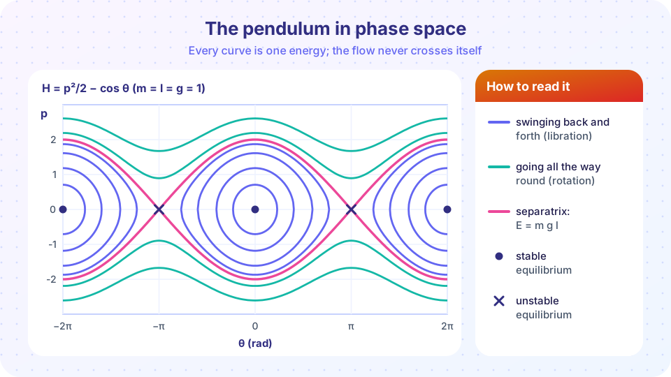
For H = p²/(2ml²) − mgl cosθ the portrait (in units where m = l = g = 1) has three regions:
- Libration (swinging). For
−mgl < E < mgl, the level curves are closed loops around the stable equilibrium(θ, p) = (0, 0). - Rotation. For
E > mglthe pendulum goes over the top and keeps circling. The curve is wavy and runs from left to right (or right to left) forever;θkeeps increasing. - Separatrix. At exactly
E = mglthe curvep = ±2cos(θ/2)passes through the unstable equilibriaθ = ±π. A pendulum on it takes infinitely long to reach the top: it is the dividing line between swinging and rotating.
The points (±π, 0) are unstable: nearby curves are pushed away. The point (0, 0) is stable: nearby curves circle it.
Liouville's theorem
Imagine many copies of a system, starting at nearby states that fill a small region of phase space. As time passes, each point follows Hamilton's equations, and the region moves and deforms. The area of the region does not change.
Proof for one degree of freedom. Hamilton's equations define a velocity field (q̇, ṗ) = (∂H/∂p, −∂H/∂q). A region's area changes at a rate given by the divergence of this field:
∂q̇/∂q + ∂ṗ/∂p = ∂²H/∂q∂p − ∂²H/∂p∂q = 0
The mixed second derivatives of a smooth function are equal, so the divergence is zero. A flow with zero divergence is incompressible. The same argument works with n pairs: the divergence is a sum of such cancelling terms, so the 2n-dimensional volume is conserved.
The shape can change dramatically. In a nonlinear system, a round blob is stretched into a long, thin filament, and shorter-period parts shear away from longer-period parts. But the area stays the same.
Two consequences:
- No attractors in Hamiltonian systems. A region cannot shrink onto a point or a curve. That is why dissipation (friction) is needed to make something settle down.
- Statistical mechanics. A probability cloud in phase space keeps its density along the flow, the starting point of equilibrium statistical mechanics.
If you add friction, for example ṗ = −∂H/∂q − γp, the divergence becomes −γ, so areas shrink as e^(−γt). That formula is a good check of the theorem: it is not magic, it is exactly the divergence.
Common misconceptions
- "Liouville means the shape of a cloud stays the same." No. Only its area (volume) stays the same; shapes shear and stretch.
- "Phase space is the same as ordinary space." No. A point of phase space is a whole state, positions and momenta together.
- "Trajectories can cross at the equilibrium points." The separatrix seems to cross itself at
(±π, 0), but those points are themselves trajectories (rest states), and the other curves approach them only ast → ±∞.
Try it
The first TryIt draws the pendulum portrait with matplotlib: the contour lines of H, the flow arrows from θ̇ = p, ṗ = −sinθ (units with m = l = g = 1), and the separatrix E = 1 in pink.
Press Run (or Ctrl + Enter) to see the result here.
Program input · what you'd type while the program runs
Type the answers before you press Run, one per line. Each time the program reads a line (with input()), it gets the next line from this box.
The second TryIt tests Liouville's theorem. It starts with a small disk of initial states around (θ, p) = (1.0, 0) (units with m = l = g = 1), moves every boundary point with a Runge-Kutta integrator and measures the area by the shoelace formula. The area stays at π·0.3² even as the shape is sheared. A second run adds friction −γp with γ = 0.3, and the area must then shrink by e^(−γt). This is a numerical experiment with a finite polygon, so the last digits are approximate.
Press Run (or Ctrl + Enter) to see the result here.
Program input · what you'd type while the program runs
Type the answers before you press Run, one per line. Each time the program reads a line (with input()), it gets the next line from this box.
The last TryIt is an interactive version. Move the slider to choose a starting angle and watch the state travel around its energy curve. This is a model in dimensionless units (m = l = g = 1), not a measurement.
Check your understanding
Quick check · 5 questions
of 5 answered You scored / 5 · perfect!
-
1. Why can two phase-space trajectories not cross (for time-independent H)?
Hamilton's equations are first order, so a point (q, p) determines the whole trajectory. A crossing would have two futures. -
2. In the pendulum portrait, what does the separatrix E = mgl represent?
At E = mgl the pendulum approaches the unstable upright position and takes infinite time to arrive. -
3. What is ∂q̇/∂q + ∂ṗ/∂p for a Hamiltonian system?
∂²H/∂q∂p − ∂²H/∂p∂q = 0, so the flow is incompressible. -
4. What happens to a phase-space area under a damped flow with ṗ = −∂H/∂q − γp?
The divergence of the flow is −γ, so area scales as e^(−γt). -
5. For E > mgl the pendulum's phase curve is...
That is rotation: the pendulum swings over the top again and again.
Summary
- A phase-space point
(q, p)is a complete state; trajectories follow level curves ofHand never cross. - The pendulum portrait has libration loops, rotation waves and a separatrix through the unstable equilibria.
- Liouville's theorem: Hamilton's flow has zero divergence, so phase-space area (volume) is preserved.
- With friction the area shrinks as
e^(−γt); this is how dissipation differs from Hamiltonian motion.
Track your progress
Create a free account to tick off lessons and pick up where you left off on any device.
of Classical Mechanics: Lagrangian and Hamiltonian lessons completed