


















Lesson 44 of 44 · Projects and Practice
Further Study: Where Lagrangian Mechanics Leads
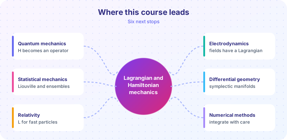
A map of the next steps after this course: quantum mechanics, statistical mechanics, relativity, field theory, differential geometry and numerical methods.
You have reached the end of the course, and you now speak the language in which most of modern physics is written. The Lagrangian and Hamiltonian formulations are not just a different way to do Newtonian mechanics. They are the form that survives when the physics changes: for quantum mechanics, relativity, fields and statistical systems, the starting point is still a Lagrangian or a Hamiltonian.
This last lesson shows where each idea of the course reappears, and what to read or study next.
What you will learn
- Which idea of this course carries over to each follow-up subject.
- A reasonable order in which to study them.
- Two small experiments that point toward quantum and field theory.
Six next steps
- Quantum mechanics (
/quantum-mechanics). The Hamiltonian becomes an operator, and the Poisson bracket becomes a commutator:{f, g} → [f̂, ĝ]/(iħ). The canonical pair(q, p)of this course is exactly the pair of position and momentum operators. The action returns in Feynman's path integral, where every path contributes with phasee^{iS/ħ}and the classical path is the one where the phases agree. For a deeper treatment, see/advanced-quantum-mechanics. - Statistical mechanics (
/statistical-mechanics). Liouville's theorem is the foundation of the microcanonical ensemble: a cloud of states in phase space keeps its volume, so equilibrium states are uniform on energy surfaces. Canonical transformations and action-angle variables lead to ergodic theory and chaos. - Relativity (
/relativity). A relativistic free particle hasL = −mc²√(1 − v²/c²). The same Euler-Lagrange equations produce the relativistic momentump = γmv. General relativity itself comes from an action, the Einstein-Hilbert action. - Electrodynamics and fields (
/electrodynamics). Replace the finitely many coordinatesqᵢ(t)by a fieldφ(x, t)andLby a Lagrangian density. The chain of masses in chapter 8 turns into a vibrating string as the number of masses grows, and Noether's theorem gives the conserved energy-momentum and charge of every field theory. - Differential geometry (
/differential-geometry). Phase space is a symplectic manifold, the Poisson bracket is a geometric structure, and the Lagrangian of a free particle in curved space gives geodesics. This is the setting for modern geometric mechanics. - Numerical methods (
/numerical-methods). The symplectic integrators of chapter 9 are the starting point for long simulations in celestial mechanics and molecular dynamics. Also review/differential-equationsand/linear-algebra; the eigenvalue problems of chapter 8 are everywhere.
A sensible order for most readers: linear algebra and differential equations first if you feel unsure about them; then quantum mechanics and relativity (they use the most ideas from this course); then fields, statistical mechanics and geometry.
Two small experiments
The first TryIt shows the principle behind all of this: the action is stationary on the real path. A ball is thrown up and returns to the ground after T = 2 s (m = 1 kg, g = 9.81 m/s²). The true path is z(t) = ½ g t (T − t). Add a smooth variation ε sin(πt/T) that keeps the endpoints, compute the action S = ∫(½mż² − mgz) dt numerically, and see that S has its minimum at ε = 0. For this system the exact result is S(ε) = S(0) + (mπ²/4T) ε², with no linear term. (Real paths make the action stationary, not always minimal. Here the stationary point happens to be a minimum because the potential is linear in z.)
Press Run (or Ctrl + Enter) to see the result here.
Program input · what you'd type while the program runs
Type the answers before you press Run, one per line. Each time the program reads a line (with input()), it gets the next line from this box.
The second TryIt points toward field theory. Take a chain of N masses (m = 1 kg, k = 1 N/m, spacing a = 1 m) with fixed ends. Its normal frequencies are ωₙ = 2√(k/m) sin(nπ/(2(N + 1))). For long wavelengths this becomes a straight line, ω ≈ c·κ with wave number κ: the dispersion relation of sound in a string. The plot compares the exact chain with that continuum approximation. The lattice formula is exact for this model, and the straight line is the limit of long waves.
Press Run (or Ctrl + Enter) to see the result here.
Program input · what you'd type while the program runs
Type the answers before you press Run, one per line. Each time the program reads a line (with input()), it gets the next line from this box.
Check your understanding
Quick check · 4 questions
of 4 answered You scored / 4 · perfect!
-
1. In quantum mechanics, the Poisson bracket is replaced by...
{f, g} → [f̂, ĝ]/(iħ), Dirac's rule. -
2. Which theorem in this course is the foundation of statistical mechanics?
It says phase-space volume is preserved by the flow, which underlies the microcanonical ensemble. -
3. What replaces the generalized coordinates qᵢ(t) in field theory?
A field has one degree of freedom at each point of space. -
4. In the action experiment, S(ε) − S(0) grows like...
The first variation vanishes on the real path; the second variation is positive, giving the ε² term.
Summary
- The Lagrangian and Hamiltonian forms carry over to quantum mechanics, relativity, fields, statistical mechanics and geometry.
- The action is stationary on real paths; brackets become commutators; Liouville's theorem leads to statistical mechanics.
- Continue with the follow-up tracks listed here, or return to the course home page to revisit any lesson.
Track your progress
Create a free account to tick off lessons and pick up where you left off on any device.
of Classical Mechanics: Lagrangian and Hamiltonian lessons completed