


















Lesson 26 of 44 · Hamiltonian Mechanics
The Legendre Transform and Hamilton's Equations
Turn a Lagrangian into a Hamiltonian step by step with the Legendre transform, derive Hamilton's equations and apply them to oscillators, pendulums and charged particles.
Lagrange's equations are second-order differential equations in the coordinates. They work, but they hide a symmetry: coordinates and momenta play very different roles in them. Hamilton's idea was to treat position and momentum as two independent variables of equal standing. To do that, you need a function that depends on q and p instead of q and q̇. The mathematical tool is the Legendre transform.
In this lesson you learn the transform from a picture, derive Hamilton's equations from it in four lines, and then apply the recipe to four systems, including a charged particle in a magnetic field, where the answer is not simply "T plus V".
What you will learn
- What the Legendre transform does geometrically and algebraically.
- How to get
H(q, p, t)fromL(q, q̇, t)with a four-step recipe. - How to derive Hamilton's equations.
- When
Hequals the total energy, and how it looks for a charged particle.
Key terms
Conjugate momentum: p = ∂L/∂q̇.
Hamiltonian: H(q, p, t) = Σ pᵢq̇ᵢ − L, written as a function of q, p and t.
Hamilton's equations: q̇ = ∂H/∂p, ṗ = −∂H/∂q.
Legendre transform: swapping a function of a variable for a function of its slope.
The Legendre transform in one picture
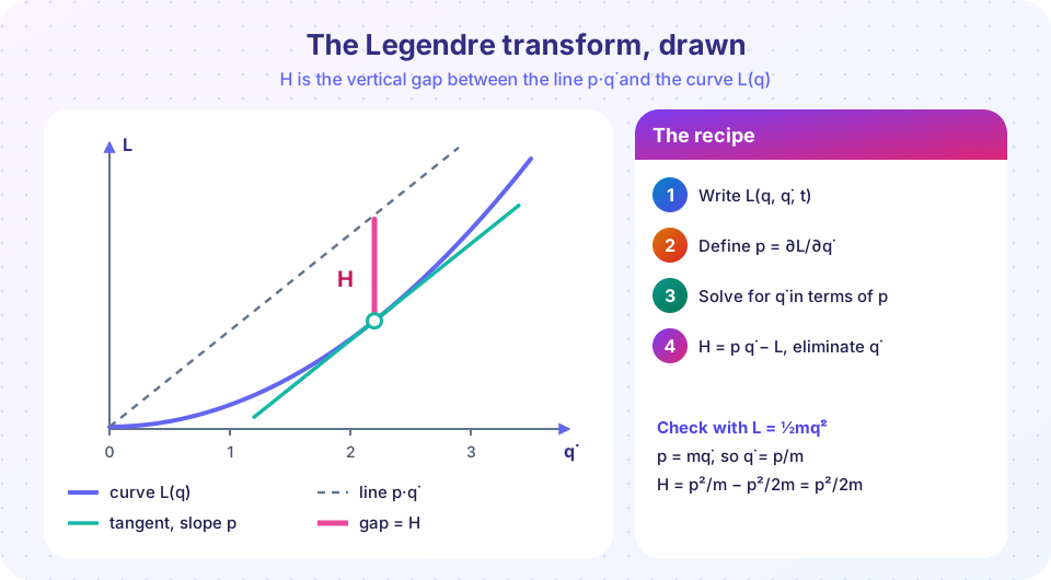
Look at a function L(v) of one variable v (here v = q̇). Its slope at a point is p = dL/dv. Draw the tangent line there, and draw the line p·v through the origin with the same slope. At the tangent point, the vertical gap between the line p·v and the curve L(v) is
H = p v − L(v)
The Legendre transform says: describe the curve by its slope p and this gap H, instead of by the point (v, L). For a convex curve (one that bends upward), each slope p belongs to exactly one point, so H is a well-defined function of p.
For L = ½mv²: the slope is p = mv, so v = p/m, and
H = p·(p/m) − ½m(p/m)² = p²/m − p²/2m = p²/2m
You have just recovered the kinetic energy written in terms of momentum.
The recipe
- Write
L(q, q̇, t). - Define the momenta
pᵢ = ∂L/∂q̇ᵢ. - Solve those equations for the velocities
q̇ᵢas functions of(q, p, t). - Compute
H = Σ pᵢq̇ᵢ − Land replace everyq̇by the expression from step 3.
Step 3 is the one that can fail: you need the velocity equations to be solvable. For ordinary mechanical systems, where L is quadratic in the velocities with a positive-definite kinetic matrix, it always works.
Deriving Hamilton's equations
Take the total differential of H = p q̇ − L(q, q̇, t):
dH = q̇ dp + p dq̇ − (∂L/∂q) dq − (∂L/∂q̇) dq̇ − (∂L/∂t) dt
Since p = ∂L/∂q̇, the dq̇ terms cancel:
dH = q̇ dp − (∂L/∂q) dq − (∂L/∂t) dt
On the other hand, H(q, p, t) has differential dH = (∂H/∂q) dq + (∂H/∂p) dp + (∂H/∂t) dt. Comparing coefficients:
q̇ = ∂H/∂p, ∂H/∂q = −∂L/∂q, ∂H/∂t = −∂L/∂t
The Euler-Lagrange equation says ṗ = ∂L/∂q, so the middle result becomes
ṗ = −∂H/∂q
Those are Hamilton's equations: q̇ = ∂H/∂p and ṗ = −∂H/∂q. There are 2n of them, each of first order. Also, dH/dt = ∂H/∂t, because along real motion ∂H/∂p · ṗ + ∂H/∂q · q̇ = −q̇ṗ + ṗq̇ = 0. So H is conserved if it has no explicit time dependence, in agreement with the energy function of the last chapter.
Examples
Harmonic oscillator. L = ½mẋ² − ½kx², p = mẋ, H = p²/2m + ½kx². Hamilton's equations: ẋ = p/m, ṗ = −kx.
Pendulum. L = ½ml²θ̇² + mgl cosθ, p_θ = ml²θ̇, H = p_θ²/(2ml²) − mgl cosθ. Equations: θ̇ = p_θ/(ml²), ṗ_θ = −mgl sinθ.
Central force. In polar coordinates H = p_r²/2m + p_θ²/(2mr²) + V(r). Because θ is missing, ṗ_θ = 0; the angular momentum is conserved and H splits into a radial problem with a centrifugal term.
A charged particle in an electromagnetic field. With charge q, scalar potential φ and vector potential A,
L = ½m v² − qφ + q A·v
The momentum is p = mv + qA, which is not just mv. Solving gives v = (p − qA)/m, and
H = (p − qA)² / 2m + qφ
The magnetic field does no work, so it adds nothing to H by itself; it enters by shifting the momentum. This p − qA structure is the one used in quantum mechanics for charged particles.
If you hold on to one fact: the Hamiltonian is not "T + V in new clothes". It is T + V for simple cases, but it is defined by the Legendre transform, and the transform tells you what to write when velocities and momenta differ.
When is H the energy?
From the last chapter, the energy function is h = Σ q̇p − L. The Hamiltonian is the same number written in different variables: H(q, p, t) = h(q, q̇(q, p, t), t). So H equals T + V exactly when h does: when the coordinates do not depend explicitly on time (the kinetic energy is purely quadratic in velocities).
Common misconceptions
- "
pis alwaysmv." Not in general: for generalized coordinatesp = ∂L/∂q̇can be an angular momentum, and with a magnetic fieldp = mv + qA. - "
HandLare the same information in different clothes, so anyLhas anH." If the velocity equations cannot be solved (singular Lagrangians, such as gauge theories) you need extra care. - "You must first write
Hin terms ofq̇." No.Hmust be expressed withqandponly. A formula withq̇in it is the energy functionh, not the Hamiltonian.
Try it
The first TryIt automates the recipe with sympy: it computes the momenta, solves for the velocities, builds H and prints Hamilton's equations. It applies the recipe to the oscillator, the pendulum and a charged particle in a uniform magnetic field B in the plane (symmetric gauge A = (−By/2, Bx/2)). This is a symbolic calculation, so the output is exact.
Press Run (or Ctrl + Enter) to see the result here.
Program input · what you'd type while the program runs
Type the answers before you press Run, one per line. Each time the program reads a line (with input()), it gets the next line from this box.
The second TryIt integrates Hamilton's equations for the pendulum (m = 1 kg, l = 1 m, g = 9.81 m/s²) with scipy and measures the period for three starting angles. The small-angle prediction 2π√(l/g) is only an approximation, and the plot shows how much the real period grows with amplitude.
Press Run (or Ctrl + Enter) to see the result here.
Program input · what you'd type while the program runs
Type the answers before you press Run, one per line. Each time the program reads a line (with input()), it gets the next line from this box.
Check your understanding
Quick check · 5 questions
of 5 answered You scored / 5 · perfect!
-
1. For L = ½mẋ² − V(x), what is the Hamiltonian?
p = mẋ so ẋ = p/m, and H = pẋ − L = p²/m − p²/2m + V = p²/2m + V. -
2. What does Hamilton's second equation say?
The sign is minus: ṗ = −∂H/∂q, and q̇ = +∂H/∂p. -
3. For a charged particle in a vector potential A, the momentum conjugate to position is...
L = ½mv² − qφ + qA·v, so p = ∂L/∂v = mv + qA. -
4. The pendulum's Hamiltonian is H = p²/(2ml²) − mgl cosθ. What is dp/dt?
ṗ = −∂H/∂θ = −mgl sinθ. -
5. Why does the Hamiltonian have to be written without q̇?
Hamilton's equations take derivatives with respect to q and p, so q̇ has to be eliminated using p = ∂L/∂q̇.
Summary
- The Legendre transform replaces
L(q, q̇)byH(q, p) = Σ pq̇ − L, withp = ∂L/∂q̇. - Hamilton's equations
q̇ = ∂H/∂p,ṗ = −∂H/∂qare2nfirst-order equations. HequalsT + Vfor time-independent constraints, but with a vector potentialp = mv + qAandH = (p − qA)²/2m + qφ.- If
Hhas no explicit time dependence, it is conserved.
Track your progress
Create a free account to tick off lessons and pick up where you left off on any device.
of Classical Mechanics: Lagrangian and Hamiltonian lessons completed