


















Lesson 16 of 44 · Lagrangian Mechanics
Lagrangian Mechanics Overview: The Five-Step Recipe
Preview Lagrangian mechanics: the five-step recipe from coordinates to equations of motion, tested on a harmonic oscillator and a free particle in polar coordinates.
Everything so far was preparation. You know how to choose generalized coordinates (chapter 1), you know where Newton's method struggles (chapter 2), and you know how to find the function that makes an integral stationary (chapter 3). Chapter 4 puts the pieces together. We apply the Euler-Lagrange equation with the integral ∫ L dt, where L = T − V, and out come the equations of motion, with no constraint forces in sight.
What you will learn
- The five-step recipe used in every Lagrangian problem.
- How Hamilton's principle links the recipe to the calculus of variations.
- How to automate the recipe in SymPy.
- What the next four lessons cover.
Key terms. The Lagrangian is L(q, q̇, t) = T − V. The action is S = ∫ L dt. Hamilton's principle: the true motion between two configurations makes S stationary. The Lagrange equations are d/dt(∂L/∂q̇ᵢ) − ∂L/∂qᵢ = 0.
Hamilton's principle in one paragraph
Fix the configuration of the system at two times, t₁ and t₂. Out of all the ways to get from one to the other, the system follows the path that makes the action S = ∫ₜ₁ᵗ² L dt stationary. Replace x → t, y → qᵢ(t) in the Euler-Lagrange equation of chapter 3 and you get one Lagrange equation for each coordinate:
d/dt (∂L/∂q̇ᵢ) − ∂L/∂qᵢ = 0 i = 1, …, n
Lesson 4.2 shows that this agrees with Newton's second law, so the principle is a new way of stating the same physics, not a new law.
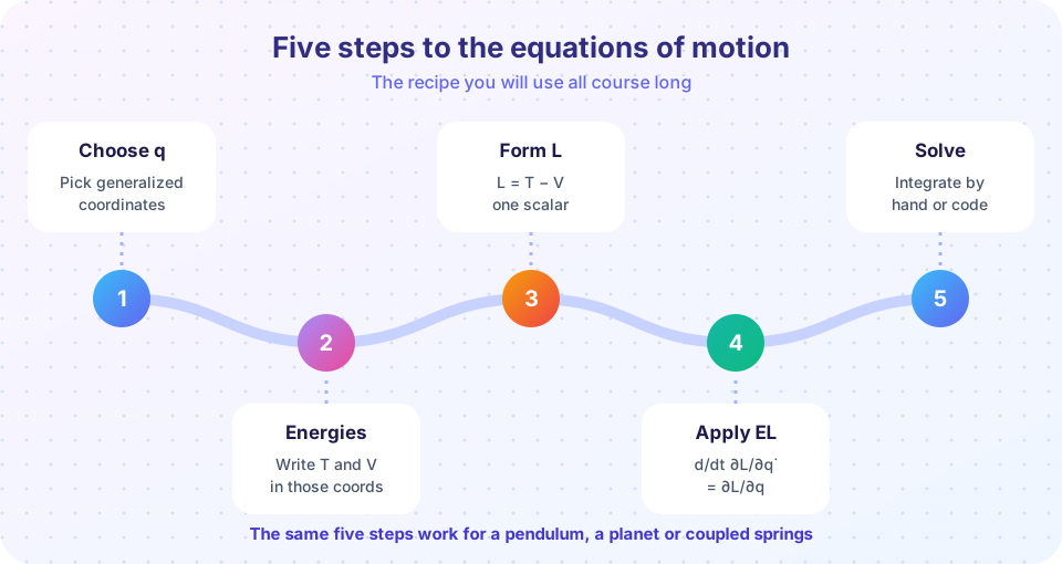
The recipe
Step 1: choose q
Steps 2 and 3: energies
Steps 4 and 5: solve
- Choose generalized coordinates
q₁ … qₙ, one per degree of freedom. - Write
Tas a function of theqandq̇(userᵢ(q, t)and the chain rule). - Write
Vas a function of theq, and formL = T − V. - Differentiate
Lto get∂L/∂q̇ᵢand∂L/∂qᵢ, then apply the Lagrange equation for eachi. - Solve the
nsecond-order equations, analytically or numerically.
The steps are mechanical. Almost all the thinking goes into step 1 (the coordinates) and the algebra of T in step 2.
Try it
A tiny helper function that carries out step 4 can be reused for every example in this chapter. Here it solves a harmonic oscillator and a free particle in polar coordinates (r, θ). Notice that the polar example produces the centripetal term r θ̇² and conservation of angular momentum with no vector algebra.
Press Run (or Ctrl + Enter) to see the result here.
Program input · what you'd type while the program runs
Type the answers before you press Run, one per line. Each time the program reads a line (with input()), it gets the next line from this box.
The same equation of motion, solved numerically for the oscillator, matches the exact cosine.
Press Run (or Ctrl + Enter) to see the result here.
Program input · what you'd type while the program runs
Type the answers before you press Run, one per line. Each time the program reads a line (with input()), it gets the next line from this box.
In this chapter
- From D'Alembert's Principle to Lagrange's Equations: why the equations agree with Newton's second law.
- Worked Examples: Atwood Machine and Rotating Hoop: the recipe on real problems.
- Generalized Momentum and Velocity-Dependent Potentials: momentum conjugate to a coordinate, and the Lorentz force.
- Chapter 4 Review.
Check your understanding
Quick check · 4 questions
of 4 answered You scored / 4 · perfect!
-
1. What is the Lagrangian of a system with kinetic energy T and potential energy V?
L = T − V; the sum T + V is the total energy. -
2. How many Lagrange equations does a system with n degrees of freedom have?
One equation for each generalized coordinate. -
3. What does Hamilton's principle say?
That is the variational statement from which the Lagrange equations follow. -
4. In the polar-coordinate free particle, what does the θ equation say?
d/dt(m r² θ̇) = 0 is conservation of angular momentum.
Summary
- Hamilton's principle plus the calculus of variations gives
d/dt(∂L/∂q̇ᵢ) − ∂L/∂qᵢ = 0. - The five steps: choose
q, writeT, writeV, apply the equations, solve. - A small SymPy helper carries out step 4, and numerical solvers carry out step 5.
Track your progress
Create a free account to tick off lessons and pick up where you left off on any device.
of Classical Mechanics: Lagrangian and Hamiltonian lessons completed