


















Lesson 9 of 47 · Numerical Foundations
Roots and Linear Systems
Solve f(x) = 0 with bisection, Newton and SciPy, apply it to Kepler's equation, and solve linear systems such as circuits with numpy.linalg.solve and condition numbers.
Many physics questions end in an equation you cannot rearrange. At what angle does a ball hit a given target? At what energy does a quantum well hold a bound state? Where is an orbiting planet at time t? Each asks for a number x such that f(x) = 0, a root of f. Others lead to many equations at once, A x = b, which is a linear system: Kirchhoff's laws for a circuit, the balance of forces in a truss.
This lesson gives you the standard tools for both, and the warning signs that tell you when to be careful.
What you will learn
- Bracket a root and find it with bisection.
- Newton's method: when it is fast and when it fails.
- Use
scipy.optimizefor robust root finding. - Solve
A x = band read the condition number.
Key terms
Root: a value x with f(x) = 0.
Bracket: an interval [a, b] where f(a) and f(b) have opposite signs, so a continuous f must cross zero inside.
Convergence order: how fast the error shrinks per step; Newton's is quadratic, bisection's is linear.
Condition number κ(A): the factor by which relative errors in b can be magnified in the solution x.
Bisection: slow, sure, simple
If f is continuous and f(a) and f(b) have opposite signs, a root lies in between. Evaluate the midpoint m = (a + b)/2; keep the half whose ends still have opposite signs. Each step halves the bracket, so after n steps the root is known to within (b − a)/2^n. To get from a bracket of width 1 to 1e-12 takes about 40 steps. Bisection needs no derivative and cannot fail once bracketed, but it cannot go faster.
Newton's method: fast, with conditions
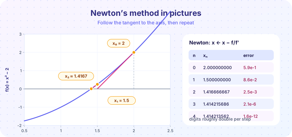
Newton replaces f by its tangent line at the current guess and jumps to where the tangent crosses zero:
x_{n+1} = x_n − f(x_n) / f′(x_n)
Near a simple root, the error roughly squares each step (quadratic convergence): 1e-2, 1e-4, 1e-8, 1e-16. The figure above shows the first iterations for f(x) = x² − 2.
Newton can fail. If f′ is near zero, the tangent is almost flat and the next guess flies away. If the starting point is far from the root, it may cycle or converge to a different root. Real codes therefore combine Newton-like speed with a bracket as a safety net, which is what scipy.optimize.brentq does.
Press Run (or Ctrl + Enter) to see the result here.
Program input · what you'd type while the program runs
Type the answers before you press Run, one per line. Each time the program reads a line (with input()), it gets the next line from this box.
A physics example: Kepler's equation
A planet on an elliptical orbit with eccentricity e obeys Kepler's equation M = E − e sin E, where M is the mean anomaly (proportional to time since perihelion) and E is the eccentric anomaly, an angle that locates the planet. Given M, you must solve for E: there is no formula. Newton's method works well, and for 0 ≤ e < 1 the function g(E) = E − e sin E − M is monotonic with g′ = 1 − e cos E > 0, so a unique root exists.
Press Run (or Ctrl + Enter) to see the result here.
Program input · what you'd type while the program runs
Type the answers before you press Run, one per line. Each time the program reads a line (with input()), it gets the next line from this box.
SciPy's tools
scipy.optimize.brentq(f, a, b) is the first choice for one variable with a bracket. root_scalar offers several methods (bisect, newton, secant, brentq), and fsolve or root handle several equations at once. Always check the success flag and the residual f(x).
Linear systems
A system of n linear equations in n unknowns is A x = b with an n × n matrix A. Example: a two-loop circuit with resistors R1 = 10 Ω, R2 = 20 Ω, a shared R3 = 30 Ω, and sources 12 V and 5 V in the loops. Writing Kirchhoff's voltage law around the two loops gives
(R1 + R3) I1 − R3 I2 = 12
−R3 I1 + (R2 + R3) I2 = −5
In matrix form A = [[40, −30], [−30, 50]], b = [12, −5]. Solve it with np.linalg.solve(A, b). Never compute inv(A) @ b: it is slower and less accurate.
Conditioning
Some systems are intrinsically sensitive. The condition number κ(A) = ‖A‖ ‖A⁻¹‖ measures how much a relative error in b (or in A) can be amplified in x. A rule of thumb: you lose about log10 κ digits. With doubles (16 digits), κ ≈ 1e10 leaves about 6 trustworthy digits. The Hilbert matrix, A_ij = 1/(i + j + 1), is a famous ill-conditioned example.
Press Run (or Ctrl + Enter) to see the result here.
Program input · what you'd type while the program runs
Type the answers before you press Run, one per line. Each time the program reads a line (with input()), it gets the next line from this box.
For the circuit, κ is small, so the answer is reliable. For the Hilbert matrix, the error grows with the condition number even though the residual H x − b stays tiny: a small residual does not guarantee a small error when κ is large.
Common misconceptions
"Newton's method always converges." It needs a good starting guess and a derivative that is not near zero.
"If the residual is tiny, the solution is accurate." For ill-conditioned systems the residual can be tiny while x is far from the truth.
"To solve Ax = b, invert A." Direct solvers based on LU factorization are faster and more accurate than forming the inverse.
Check your understanding
Quick check · 5 questions
of 5 answered You scored / 5 · perfect!
-
1. How many bisection steps are needed to shrink a bracket of width 1 to about 1e-3?
Each step halves the width: 2^10 = 1024, so ten steps. -
2. Newton's method has quadratic convergence. If the error is 1e-3 now, a typical next error is
The error roughly squares each step. -
3. Which is a warning sign for Newton's method?
A near-flat tangent throws the next guess far away. -
4. Which call solves A x = b best?
solve uses an LU factorization and is more accurate than forming the inverse. -
5. A condition number of 1e12 in double precision means roughly
You lose about log10(kappa) = 12 of the 16 digits.
Summary
- A root of
fis found safely by bisection and quickly by Newton's method;brentqcombines both ideas. - Kepler's equation is a classic physics root-finding problem.
- Solve linear systems with
np.linalg.solve, never with the inverse. - The condition number says how many digits you lose; a small residual is not proof of accuracy.
Next: Chapter 2 Review
Track your progress
Create a free account to tick off lessons and pick up where you left off on any device.
of Computational Physics lessons completed