


















Lesson 11 of 47 · Ordinary Differential Equations
Ordinary Differential Equations: Overview
Preview chapter 3: how physics becomes ordinary differential equations, how to turn second-order equations into first-order systems, and how the methods in this chapter fit.
Newton's second law, F = m a, is an ordinary differential equation (ODE): it relates a quantity (position) to its own rate of change (velocity, acceleration). So do the equations for a circuit with a capacitor, radioactive decay, a pendulum, a planet orbiting a star, and a chemical reaction. If you can write down the forces, you can write down an ODE; if you can solve ODEs numerically, you can predict the motion even when no formula exists.
What you will learn
- What an initial value problem is and why it can be solved step by step.
- How to reduce any higher-order ODE to a first-order system.
- Where each lesson in this chapter fits.
- How to solve an ODE with
scipy.integrate.solve_ivpas a reference.
Key terms
ODE: an equation with a function of one variable (usually time) and its derivatives.
Initial value problem (IVP): an ODE together with the state at a starting time.
State vector: the list of quantities that fully describe the system at one instant, such as (x, v).
Time step h or dt: the size of each jump forward in time.
Phase space: the space of all possible state vectors.
Why step by step?
The methods in this chapter
What can go wrong
Initial value problems
A first-order IVP has the form
dy/dt = f(t, y), y(t₀) = y₀
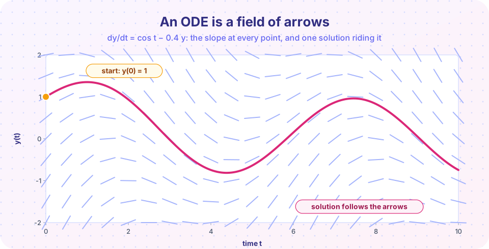
The function f gives the slope of the solution at any point. If you know where you are and which way you are heading, a short step forward gets you to a nearby point; repeating the process traces out the curve. The figure above shows such arrows for dy/dt = cos t − 0.4 y. Every numerical method in this chapter is a different way of choosing that short step.
Turning second-order equations into first-order systems
Newton's law for a mass on a spring is second order: m d²x/dt² = −k x. The methods in this chapter handle only first-order systems, so introduce the velocity v = dx/dt as a new unknown:
dx/dt = v
dv/dt = −(k/m) x
Now the state is the vector (x, v). Any ODE of order n becomes n first-order equations in the same way. This is a routine trick you will use in every lesson of this chapter.
Press Run (or Ctrl + Enter) to see the result here.
Program input · what you'd type while the program runs
Type the answers before you press Run, one per line. Each time the program reads a line (with input()), it gets the next line from this box.
Phase space
Instead of plotting x and v against time, plot them against each other. For the spring the points lie on an ellipse because the energy E = (m v² + k x²)/2 is constant. Closed curves in phase space mean periodic motion; a curve that spirals outward means energy is being created, which for a frictionless spring is a numerical error. Phase portraits are the best way to spot sick simulations.
Press Run (or Ctrl + Enter) to see the result here.
Program input · what you'd type while the program runs
Type the answers before you press Run, one per line. Each time the program reads a line (with input()), it gets the next line from this box.
What each lesson covers
- Euler's Method: the simplest step, its error and its instability.
- Runge-Kutta Methods: midpoint and RK4, and how to measure their order.
- Oscillators and Energy: leapfrog and velocity Verlet, which keep energy bounded.
- Projectile Motion with Drag: a realistic force with no closed-form solution, solved with
solve_ivp. - Chapter 3 Review: comparison table and a long quiz.
Common misconceptions
"An ODE solver gives the exact solution." It gives a sequence of approximate values. Accuracy depends on the method, the step and the problem.
"A second-order equation needs a second-order method." The order of the ODE and the order of the method are unrelated. You first rewrite the equation as a first-order system, then choose any method.
Check your understanding
Quick check · 4 questions
of 4 answered You scored / 4 · perfect!
-
1. What do you need to start solving dy/dt = f(t, y)?
An initial value problem is the ODE together with the state at the starting time. -
2. How is m x'' = -k x written as a first-order system?
Introduce v = x' as a new unknown; the second-order equation becomes two first-order ones. -
3. In phase space, a frictionless oscillator traces
Energy is conserved, so the state stays on one contour of energy. -
4. A simulated frictionless oscillator spirals outward in phase space. What does this suggest?
Real frictionless oscillators do not gain energy; the drift is a numerical artifact.
Summary
- An ODE gives the slope at every state; an IVP adds the starting state.
- Higher-order equations become first-order systems by adding velocities as unknowns.
- Phase portraits reveal energy behavior at a glance.
solve_ivpis a trustworthy reference to test your own solvers against.
Next: Euler's Method
Track your progress
Create a free account to tick off lessons and pick up where you left off on any device.
of Computational Physics lessons completed