


















Lesson 25 of 47 · Partial Differential Equations
The wave equation and the leapfrog scheme
Simulate a vibrating string with the leapfrog scheme, learn the CFL stability condition and see the numerical errors that appear when r is below one.
A plucked guitar string, a ripple on a pond and a pulse on a rope all follow the wave equation. Unlike heat, a wave does not smear out: a pulse keeps its shape and runs at a fixed speed c. That one fact changes how we must build the solver, because the numerical method must carry information at the right speed or it will fail.
What you will learn
- How the 1D wave equation and d'Alembert's solution describe a string.
- How the leapfrog scheme uses two earlier time levels.
- Why
r = cΔt/Δx ≤ 1(the CFL condition) is needed. - What numerical dispersion is and when you can see it.
Key terms
Wave speed (c): how fast a disturbance travels. For a string it is √(T/μ), tension divided by mass per length, square-rooted.
Leapfrog: a scheme that is centred in both time and space and uses u[n] and u[n−1] to compute u[n+1].
CFL condition: Courant-Friedrichs-Lewy, the requirement that information cannot skip over grid cells in one step.
Numerical dispersion: waves of different wavelengths travel at slightly different speeds on the grid, even though they should all move at c.
The equation and its exact solution
∂²u/∂t² = c² · ∂²u/∂x²
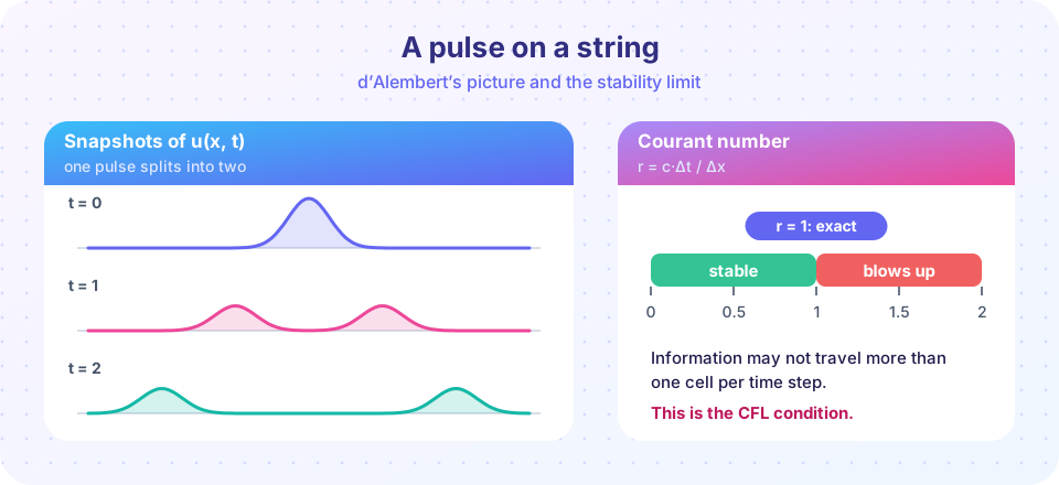
In 1750, Jean le Rond d'Alembert showed that every solution on an infinite string has the form u(x, t) = F(x − ct) + G(x + ct): one shape moving right plus one moving left. A pulse released at rest simply splits into two copies of half the height, as in the picture. A string with fixed ends then reflects them back, flipped upside down.
The leapfrog scheme
Use a central difference in time and in space:
(u[n+1,j] − 2u[n,j] + u[n−1,j]) / Δt² = c² (u[n,j+1] − 2u[n,j] + u[n,j−1]) / Δx²
Solving for the new value, with r = cΔt/Δx:
u[n+1,j] = 2u[n,j] − u[n−1,j] + r² (u[n,j+1] − 2u[n,j] + u[n,j−1])
The scheme needs two time levels to start. For a string released from rest, a Taylor expansion gives the first step:
u[1,j] = u[0,j] + ½ r² (u[0,j+1] − 2u[0,j] + u[0,j−1])
If the string starts with a speed v₀(x), add the term Δt·v₀(x_j).
Why r must not exceed 1
The true solution at (x, t + Δt) depends on the initial data in the interval [x − cΔt, x + cΔt]. The numerical value depends only on the three points x − Δx, x, x + Δx. If cΔt > Δx, the true answer needs information that the scheme never looks at. It cannot possibly be right, and it turns out to be unstable. That is the CFL condition: r ≤ 1.
A remarkable detail: at exactly r = 1, the leapfrog scheme reproduces the exact solution on the grid points (for the pure wave equation). Why not always pick r = 1 then? In real problems the wave speed changes with position (different tension or density), so r cannot be 1 everywhere. We pick Δt for the fastest region and accept r < 1 elsewhere.
Numerical dispersion
When r < 1, short wavelengths lag behind long ones. A smooth pulse develops a trailing wiggle behind it. This is an error of the grid, not the physics. It shrinks as you refine the mesh, and it is much worse for wavelengths of only a few grid points. A rule of thumb used in practice: resolve each wavelength with at least 10 to 20 points.
Common misconceptions
- "The solver is wrong because the pulse changes shape." On a coarse grid with r < 1 it does; test with a finer grid before blaming the physics.
- "The wave equation damps like the heat equation." The exact equation conserves energy. Numerical damping you see comes from the scheme.
- "Fixed ends make the string stop." Fixed ends reflect the wave and invert it; the energy stays in the string.
Try it
We release a Gaussian pulse from rest on a string with fixed ends and plot snapshots. With r = 1 they match d'Alembert's solution before the pulses reach the walls.
Press Run (or Ctrl + Enter) to see the result here.
Program input · what you'd type while the program runs
Type the answers before you press Run, one per line. Each time the program reads a line (with input()), it gets the next line from this box.
Now we try three values of r and record the largest displacement after the same physical time.
Press Run (or Ctrl + Enter) to see the result here.
Program input · what you'd type while the program runs
Type the answers before you press Run, one per line. Each time the program reads a line (with input()), it gets the next line from this box.
A third experiment looks at dispersion. A narrow pulse on a coarse grid with r = 0.5 leaves ripples behind; we measure the size of the largest ripple.
Press Run (or Ctrl + Enter) to see the result here.
Program input · what you'd type while the program runs
Type the answers before you press Run, one per line. Each time the program reads a line (with input()), it gets the next line from this box.
Check your understanding
Quick check · 5 questions
of 5 answered You scored / 5 · perfect!
-
1. d'Alembert's solution of the 1D wave equation is...
Every solution is a right-moving shape plus a left-moving shape. -
2. The leapfrog scheme needs which time levels to compute u[n+1]?
The second time derivative uses three levels: n−1, n and n+1. -
3. With c = 340 m/s and Δx = 0.01 m, what is the largest stable Δt?
r = cΔt/Δx ≤ 1 gives Δt ≤ Δx/c = 0.01/340 ≈ 2.9e-5 s. -
4. Why does the CFL condition exist?
If a wave can travel further than one cell per step, the numerical stencil misses information the true solution needs. -
5. What does numerical dispersion cause?
On the grid, short wavelengths lag, which creates ripples behind sharp pulses.
Summary
u_tt = c²·u_xxhas solutionsF(x − ct) + G(x + ct); a pulse splits into two travelling halves.- Leapfrog:
u[n+1] = 2u[n] − u[n−1] + r²·(second difference), started with a special first step. - Stability requires
r = cΔt/Δx ≤ 1(the CFL condition);r = 1is exact for the plain 1D equation. - With
r < 1, numerical dispersion shows up as ripples; refine the grid to reduce them.
Track your progress
Create a free account to tick off lessons and pick up where you left off on any device.
of Computational Physics lessons completed