


















Lesson 34 of 47 · Quantum Simulations
Energy levels from matrices
Solve the 1D time-independent Schrödinger equation with a finite-difference matrix and scipy: particle in a box, harmonic oscillator and a finite well, with error checks.
An electron trapped in a tiny region cannot have just any energy. Only certain levels are allowed, and each comes with its own standing-wave shape. Finding them analytically works for a few potentials. For the rest, the trick is to turn the differential equation into a matrix, because computers are superb at matrices. Once you can do this you can compute the spectrum of almost any one-dimensional potential, from a quantum dot to the stretching of a diatomic molecule.
What you will learn
- How the second derivative becomes a tridiagonal matrix.
- How to compute energies and wave functions with
scipy.linalg.eigh_tridiagonal. - How to check numerical levels against exact results for the box and the oscillator.
- How the error shrinks when the grid is refined.
Key terms
Eigenvalue / eigenvector: for a matrix H, a number E and vector ψ with Hψ = Eψ.
Tridiagonal matrix: a matrix whose only non-zero entries lie on the diagonal and the two neighboring diagonals.
Ground state: the lowest-energy eigenstate.
Node: a point where the wave function crosses zero; the n-th state has n − 1 nodes in a box.
Bound state: an eigenstate whose probability stays localized, with energy below the potential at infinity.
From derivative to matrix
Put the particle on a grid x_j = x_0 + jΔx. The second derivative at each point is
ψ''(x_j) ≈ (ψ_{j+1} − 2ψ_j + ψ_{j−1}) / Δx²
so in natural units, Hψ = Eψ becomes, for each j,
−(1/(2Δx²)) ψ_{j−1} + (1/Δx² + V_j) ψ_j − (1/(2Δx²)) ψ_{j+1} = E ψ_j
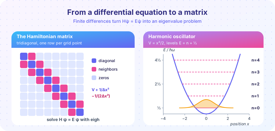
That is a matrix equation. The matrix H has 1/Δx² + V_j on the diagonal and −1/(2Δx²) on the two neighboring diagonals, as in the picture. Its eigenvalues are approximations to the energy levels, and each eigenvector, after dividing by √Δx, is the sampled wave function, normalized so that Σ|ψ_j|² Δx = 1.
Boundary conditions come for free: if the grid ends where ψ should be zero (the walls of a box, or far out where a bound state has decayed), we just leave those values out.
The eigenvalues of a symmetric tridiagonal matrix can be found extremely fast. eigh_tridiagonal(diag, off, select="i", select_range=(0, k)) returns only the lowest k + 1 of them.
Three tests with known answers
- Particle in a box of length 1 (walls at 0 and 1,
V = 0inside):E_n = n²π²/2 ≈ 4.935, 19.74, 44.41, …. - Harmonic oscillator
V = x²/2:E_n = n + ½:0.5, 1.5, 2.5, …. The levels are evenly spaced. - Finite square well of depth
V0and half-widtha: even states satisfyk tan(ka) = κwithk = √(2E),κ = √(2(V0 − E)). Unlike the box, the wave function leaks into the walls, so the energies are lower than the box's.
Common misconceptions
- "Any grid will do." A grid that is too coarse blurs the high states, and a domain that is too narrow squeezes a bound state into an artificial box.
- "Eigenvectors from eigh are probabilities." The probability density is the eigenvector squared (and divided by Δx); the vector itself can be positive or negative.
- "The numerical levels are all accurate." Accuracy drops for high levels, whose wave function oscillates faster and is resolved by fewer points.
- "The sign of an eigenvector matters."
ψand−ψdescribe the same state.
Try it
First, the box and the oscillator. We print numerical energies next to exact ones.
Press Run (or Ctrl + Enter) to see the result here.
Program input · what you'd type while the program runs
Type the answers before you press Run, one per line. Each time the program reads a line (with input()), it gets the next line from this box.
Next, convergence. The error of the lowest box level should shrink like Δx²: doubling the number of points cuts it by about four.
Press Run (or Ctrl + Enter) to see the result here.
Program input · what you'd type while the program runs
Type the answers before you press Run, one per line. Each time the program reads a line (with input()), it gets the next line from this box.
Finally the finite well. We compute its ground state numerically and compare it with the root of the transcendental equation k tan(ka) = κ.
Press Run (or Ctrl + Enter) to see the result here.
Program input · what you'd type while the program runs
Type the answers before you press Run, one per line. Each time the program reads a line (with input()), it gets the next line from this box.
The two ground-state values differ by about 0.4 percent. The grid decides which points count as "inside" the well, so the numerical well is up to one cell wider or narrower than the exact one. Refining the grid closes the gap.
Check your understanding
Quick check · 5 questions
of 5 answered You scored / 5 · perfect!
-
1. What are the diagonal entries of the finite-difference Hamiltonian (natural units)?
The kinetic term contributes 1/Δx² on the diagonal (from −½·(−2/Δx²)), the potential adds V_j. -
2. What are the exact energies of a particle in a box of length 1 (ħ = m = 1)?
E_n = n²π²ħ²/(2mL²) with ħ = m = L = 1. -
3. The error of the lowest numerical level drops by about 4 when N doubles. This shows the scheme is...
Error ∝ Δx² means halving Δx divides the error by 4. -
4. In a finite well compared with an infinite box of the same width, the ground-state energy is...
The wave function leaks into the walls, so it is less confined and its energy is lower. -
5. The harmonic oscillator levels are...
E_n = (n + ½)ħω, so neighboring levels differ by ħω.
Summary
- A finite-difference Hamiltonian is a tridiagonal matrix:
1/Δx² + V_jon the diagonal and−1/(2Δx²)beside it. eigh_tridiagonalreturns the lowest eigenvalues and eigenvectors quickly; divide by√Δxto normalize.- Tests: box
E = n²π²/2, oscillatorE = n + ½, finite well fromk tan(ka) = κ. - The error shrinks like
Δx²; high levels need finer grids.
Track your progress
Create a free account to tick off lessons and pick up where you left off on any device.
of Computational Physics lessons completed