


















Lesson 5 of 47 · Getting Started
Chapter 1 Review: Getting Started
Review chapter 1 of the computational physics course: the simulation workflow, NumPy arrays, and plotting habits, with a recap table and a ten-question quiz.
You have met the three things every later chapter relies on: the workflow (question, model, algorithm, code, check), the array as the basic data type, and the plot as the way to see and check results. This review pulls them into one picture, a recap table and a quiz that mixes all the lessons.
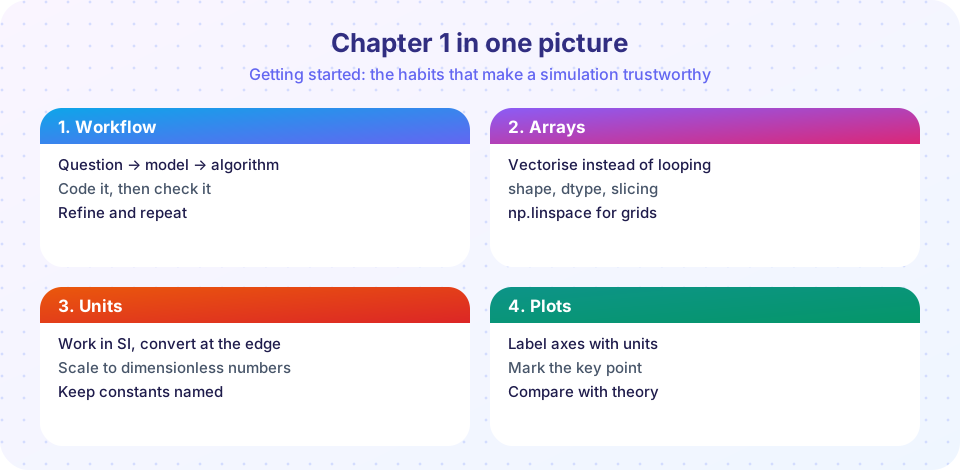
What you will review
- The five-step workflow and the verification/validation split.
- NumPy: shape,
linspace, vectorization, slices, masks, broadcasting. - Plot labeling, error bars, residuals and log axes.
Recap table
| Lesson | Core idea | One-line test of understanding |
|---|---|---|
| Course map | Nine chapters, validate everything | Why is "no error message" not proof of a right answer? |
| What is computational physics? | Loop: question, model, algorithm, code, check | What is the difference between verification and validation? |
| Python and NumPy | Vectorized array math | What shape does (4,1) + (1,5) give? |
| Plotting physics data | Units, error bars, residuals, log axes | What does a pattern in the residuals mean? |
Putting it together
The next example uses every skill from this chapter. It follows the whole loop for a small problem: how far does a ball travel when launched at 20 m/s at different angles? The model is a point mass without drag; the check compares the vectorized result with the textbook formula R = v² sin(2θ) / g.
Press Run (or Ctrl + Enter) to see the result here.
Program input · what you'd type while the program runs
Type the answers before you press Run, one per line. Each time the program reads a line (with input()), it gets the next line from this box.
The two computations agree to rounding error, so the check passes. In chapter 3 you will add drag, where no formula exists and the check changes to "turn drag to zero and recover this curve".
Chapter review quiz
Quick check · 10 questions
of 10 answered You scored / 10 · perfect!
-
1. In the workflow, which step does verification belong to?
Verification and validation are both parts of the check step. -
2. Which statement about validation is correct?
Validation compares the model with reality, for example experiments or trusted data. -
3. What does np.linspace(1, 3, 5) give?
Five evenly spaced points including both ends: step 0.5. -
4. a has shape (3, 1) and b has shape (1, 4). The shape of a * b is
Broadcasting expands size-1 axes to give (3, 4). -
5. c = a[2:5] and then c[0] = -1 changes which element of a?
A slice is a view, so c[0] is a[2]. -
6. A pendulum's period T versus length L gives a straight line of slope 0.5 on log-log axes. What does this tell you?
The slope on a log-log plot is the exponent, so T is proportional to L to the power 1/2. -
7. Which axis label is best?
Name the quantity, give its symbol, and give the unit. -
8. Residuals of a fit show a clear U-shaped pattern. What is the likely issue?
Systematic residuals mean the model is missing a feature the data contain. -
9. Why is a smaller time step not always better?
More steps mean more rounding; chapter 2 quantifies the trade-off. -
10. Which pairing of tools is most appropriate to see whether an error shrinks as a power of the step size?
A power law appears as a straight line on log-log axes, and its slope is the exponent.
Summary
- The workflow ends with a check, and verification comes before validation.
- Arrays, vectorization, slices (views), masks and broadcasting are the working tools.
- Good plots name quantities and units, show uncertainty and residuals, and use log axes for power laws.
- Chapter 2 asks the next question: how accurate can numbers on a computer be?
Track your progress
Create a free account to tick off lessons and pick up where you left off on any device.
of Computational Physics lessons completed