


















Lesson 21 of 47 · Monte Carlo Methods
The Ising Model and the Metropolis Algorithm
Simulate the 2D Ising model with the Metropolis algorithm: spins, energy, Boltzmann weights, magnetization, the phase transition at Tc = 2.269, and an interactive lattice.
Heat an iron magnet and at 770 degrees Celsius it suddenly stops being magnetic. Cool it and the magnetism returns. This sharp change is a phase transition, and the simplest model that captures it is the Ising model: a lattice of tiny arrows (spins) that prefer to point the same way as their neighbors, jostled by thermal noise. The model is also the textbook use of Metropolis Monte Carlo, a method for sampling the states of any thermal system. In one short program you can watch order appear and disappear.
What you will learn
- The Ising energy and the Boltzmann distribution.
- The Metropolis acceptance rule and why it samples the right states.
- A fast vectorized implementation with a checkerboard update.
- How magnetization, energy and heat capacity reveal the transition.
Key terms
Spin sᵢ: a variable equal to +1 or −1 on each lattice site.
Ising energy: E = −J Σ⟨ij⟩ sᵢ sⱼ, a sum over neighboring pairs; J > 0 favors alignment.
Boltzmann weight: the probability of a configuration is proportional to exp(−E / k_B T).
Magnetization per spin: m = (1/N) Σ sᵢ.
Sweep: one attempted update for each spin on average.
The model
Put a spin sᵢ = ±1 on each site of an L × L square lattice with periodic boundaries (the right edge wraps to the left, the top to the bottom, so there are no special edge sites). Each pair of nearest neighbors contributes −J sᵢ sⱼ to the energy: −J if they agree, +J if they disagree. Aligned arrangements have the lowest energy.
At temperature T the probability of a configuration is P ∝ exp(−E / k_B T). In units where J = k_B = 1, the temperature is measured in units of J/k_B. There are 2^(L²) configurations, far too many to sum over: a 20 × 20 lattice already has about 10¹²⁰. Monte Carlo samples the important ones instead.
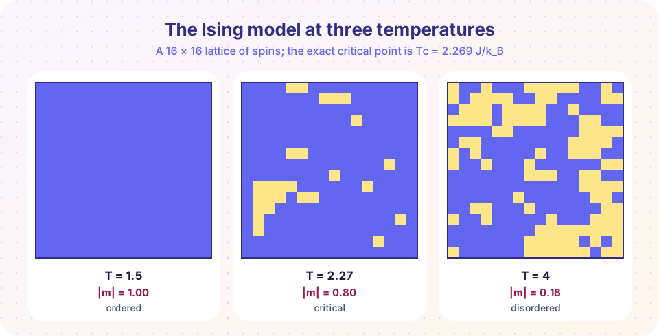
Two forces compete. Energy wants order (all spins aligned); entropy wants disorder (many more random configurations). At low T energy wins and the lattice magnetizes spontaneously, with all spins mostly up or mostly down. At high T entropy wins and the average magnetization vanishes. Between lies a critical temperature. For the 2D square lattice Onsager solved the model exactly in 1944:
T_c = 2 J / (k_B ln(1 + √2)) ≈ 2.269 J/k_B
The Metropolis algorithm
Metropolis and colleagues showed in 1953 how to walk through configurations so that each appears with its Boltzmann probability. One step:
- Pick a spin
i(at random or in a systematic order). - Compute the energy change
ΔEif it flipped. For the Ising model,ΔE = 2 J sᵢ Σ_nn sⱼ, which depends only on the four neighbors. - If
ΔE ≤ 0, accept the flip. Otherwise accept it with probabilityexp(−ΔE / k_B T). - Repeat.
The rule satisfies detailed balance, P(A) × (rate A → B) = P(B) × (rate B → A), which guarantees that long runs visit states with the right probabilities. Early in the run the lattice remembers its starting state, so discard the first sweeps as equilibration (burn-in) before measuring.
A fast implementation
A Python loop over L² spins per sweep is slow. Spins of the same checkerboard color are never neighbors, so all spins of one color can be updated at once with array operations. Updating the two colors in turn is a valid Metropolis scheme.
Press Run (or Ctrl + Enter) to see the result here.
Program input · what you'd type while the program runs
Type the answers before you press Run, one per line. Each time the program reads a line (with input()), it gets the next line from this box.
On a finite lattice the transition is rounded: below T_c the simulation follows the exact curve, above it the finite-size magnetization stays a bit above zero (about 1/L scale fluctuations). On large lattices it approaches the exact curve more sharply. Using |m| avoids the cancellation between "mostly up" and "mostly down" runs.
Energy and heat capacity
The average energy and its fluctuations also carry the transition's signature. The heat capacity per spin follows from fluctuations alone:
C = (⟨E²⟩ − ⟨E⟩²) / (N k_B T²)
It peaks near T_c: near the transition the system can absorb heat by rearranging many spins at almost no change in temperature. This peak is the numerical sign of the phase transition.
Press Run (or Ctrl + Enter) to see the result here.
Program input · what you'd type while the program runs
Type the answers before you press Run, one per line. Each time the program reads a line (with input()), it gets the next line from this box.
Play with the lattice
In the interactive lattice below, move the temperature slider and watch the domains. At low T the lattice orders; near T_c clusters of every size appear and change slowly (critical slowing down: successive samples become highly correlated, so error bars must account for it); at high T the lattice flickers randomly. The simulation uses single-spin Metropolis updates on a 48 × 48 lattice with periodic boundaries.
Why Metropolis matters beyond magnets
The same recipe samples any system whose configurations x have probability ∝ exp(−E(x)/k_B T): a gas of atoms with a pair potential, a polymer chain, a lattice gauge field in particle physics, even an optimization problem (simulated annealing). Only the proposal move and the energy function change.
Common misconceptions
"The simulation shows how spins flip in real time." Metropolis samples equilibrium states; the order of updates is a computational choice, not real dynamics (although it is often used as a model of slow dynamics).
"A finite lattice has a sharp transition." Only the infinite system does. A finite lattice has a smooth crossover; the transition sharpens as L grows.
"Averaging the signed magnetization is fine." Below T_c the lattice may be mostly up or mostly down; the signed average can cancel to zero in long runs. Use |m| or m².
"Start anywhere, measure immediately." Without equilibration the average reflects the starting state, not the temperature.
Check your understanding
Quick check · 6 questions
of 6 answered You scored / 6 · perfect!
-
1. In the Ising model with J = 1, what is the energy change when flipping a spin with neighbor sum S?
Flipping s changes the four bond energies from -s S to +s S, so dE = 2 s S. -
2. The Metropolis rule accepts an energy-raising flip with probability
Lowering moves are always accepted; raising moves with the Boltzmann factor. -
3. Which temperature is the exact 2D square-lattice critical point?
Onsager's result: Tc = 2 J / (k ln(1 + sqrt 2)). -
4. Why use periodic boundary conditions?
Edges would otherwise behave differently from the interior. -
5. What is equilibration (burn-in)?
Only after equilibration do the samples follow the Boltzmann distribution. -
6. Why does the heat capacity peak near Tc?
C is proportional to the variance of the energy, which peaks at the transition.
Summary
- The Ising energy is
E = −J Σ sᵢ sⱼ; states appear with probability∝ exp(−E / k_B T). - Metropolis flips a spin if
ΔE ≤ 0or with probabilityexp(−ΔE / k_B T). - A checkerboard update vectorizes a sweep; discard burn-in before measuring.
- Magnetization drops and heat capacity peaks near
T_c = 2.269 J/k_B. - Near
T_c, samples are strongly correlated (critical slowing down).
Next: Chapter 4 Review
Track your progress
Create a free account to tick off lessons and pick up where you left off on any device.
of Computational Physics lessons completed