


















Lesson 1 of 47 · Getting Started
Course Map: Computational Physics
See the whole computational physics course at a glance: who it is for, what you need, how to study it, and a nine-chapter map from Python basics to quantum simulations.
Physics describes nature with equations. Most of those equations cannot be solved with pencil and paper once a problem becomes realistic: a pendulum that swings through a large angle, a ball that feels air drag, a gas of a thousand interacting atoms, an electron in a strange potential well. Computational physics is the craft of turning such equations into programs, running them, and judging whether the answers deserve trust.
This course teaches that craft from the first script to molecular dynamics and quantum simulations. Every idea is shown with code that runs in your browser, so you can change a number and watch the physics respond.
What you will learn
- What the course covers and how the nine chapters connect.
- Which math, physics and Python you should already know.
- A study routine that turns reading into skill.
- How to run and modify a first simulation right here.
Key terms
Simulation: a program that follows a physical model step by step to predict behavior.
Model: the equations and assumptions that stand in for the real system.
Algorithm: a finite recipe for computing an answer from a model.
Validation: checking that a simulation agrees with known results or experiments.
Who this course is for
The course suits three kinds of reader. If you are a physics or engineering student, it fills the gap between your lecture courses and the numerical work your lab, thesis or job will demand. If you are a programmer curious about science, it shows where your skills meet real equations. If you are a teacher or self-learner, it offers a path with checkpoints, quizzes and projects.
You do not need a research background. You do need three things.
- Calculus: derivatives and integrals at the level of a first university or A level course. You should know what
dy/dtmeans. - Introductory physics: Newton's laws, energy, and the idea of a field. Chapters on quantum mechanics define everything they use.
- A little Python: variables, loops, functions and lists. Chapter 1 teaches NumPy and Matplotlib from scratch, and the Python tutorial on this site covers the language itself.
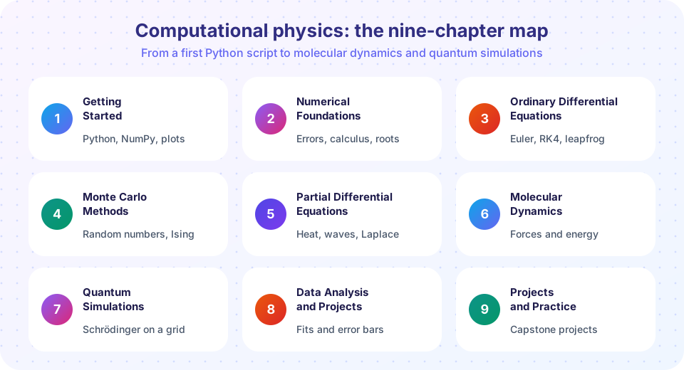
The nine chapters
Chapter 1: Getting Started
Chapter 2: Numerical Foundations
Chapter 3: Differential Equations
Chapter 4: Monte Carlo
Chapter 5: Partial Differential Equations
Chapter 6: Molecular Dynamics
Chapter 7: Quantum Simulations
Chapters 8 and 9
This first half of the course (chapters 1 to 4) gives you the numerical core: arrays, error control, time stepping and randomness. The second half applies it to fields, atoms, quantum systems and real data.
How to study this course
Reading about numerical methods is like reading about swimming. Use this routine for every lesson.
- Skim the "What you will learn" list so you know the goal.
- Read with a question in mind: what could go wrong with this method?
- Run every example, then break it. Change the step size, the starting value or the seed. Predict the effect before pressing Run.
- Write the check first. Before trusting an answer, decide what a correct answer must satisfy: a known limit, a conserved quantity, a halving test.
- Take the quiz without looking back, then reread the parts you missed.
Keep a notebook of surprises. Every time a simulation misbehaves, write down the symptom and the cause. After a few chapters this list becomes your debugging guide.
Common misconceptions
"If the program runs without errors, the answer is right." A program can run perfectly and still produce nonsense: a too-large step size, an unnoticed unit mix-up, a wrong sign. Validation is a separate step, and this course practices it from lesson one.
"A smaller step size is always better." Chapter 2 shows why not: past a point, rounding errors grow while the model error shrinks only a little.
Try it
Your first simulation: a ball dropped from 20 m. The code advances time in small steps and compares the result with the exact answer y = y0 - g t² / 2.
Press Run (or Ctrl + Enter) to see the result here.
Program input · what you'd type while the program runs
Type the answers before you press Run, one per line. Each time the program reads a line (with input()), it gets the next line from this box.
Now see how the difference depends on the step size. Each row uses a smaller step, and the code measures the height after 1.5 s.
Press Run (or Ctrl + Enter) to see the result here.
Program input · what you'd type while the program runs
Type the answers before you press Run, one per line. Each time the program reads a line (with input()), it gets the next line from this box.
Check your understanding
Quick check · 4 questions
of 4 answered You scored / 4 · perfect!
-
1. What is the main job of computational physics?
Simulation complements theory and experiment. The craft includes building, running and validating the model. -
2. Which prerequisite does the course explicitly ask for?
Calculus is needed throughout. Python is taught from basics in chapter 1 and physics concepts are defined as they appear. -
3. A program runs with no errors and prints a number. What does that prove?
Running without error says nothing about physical or numerical correctness. Checks against limits and conserved quantities are required. -
4. In the study routine, what should you do before trusting an answer?
Writing the check first, such as a known limit or a conserved quantity, keeps you honest.
Summary
- Computational physics turns equations that cannot be solved by hand into programs you can trust after checking them.
- The course has nine chapters: setup, numerics, ODEs, Monte Carlo, PDEs, molecular dynamics, quantum simulations, data analysis and projects.
- You need calculus, introductory physics and a little Python.
- Study by running, breaking and checking every example.
- Shrinking the time step reduced the error roughly in proportion to the step, and chapter 2 explains why that cannot go on forever.
Track your progress
Create a free account to tick off lessons and pick up where you left off on any device.
of Computational Physics lessons completed