


















Lesson 36 of 47 · Quantum Simulations
The variational method
Use the variational principle to bound a ground-state energy: trial Gaussians for the quartic oscillator and hydrogen, plus a Monte Carlo local-energy estimate.
When a quantum system has no exact solution, you can still ask for something very useful: a number you can trust to be above the true ground-state energy. The variational principle gives exactly that. You guess a shape for the wave function, leave a parameter free, and let the computer find the best value. The result is never below the truth, and a good guess lands very close to it. Chemists use this idea to compute the energies of molecules every day; physicists use it for helium, for superfluids and for nuclei.
What you will learn
- The variational principle and why it holds.
- How to evaluate
E(α) = ⟨ψ|H|ψ⟩ / ⟨ψ|ψ⟩analytically and numerically. - How a one-parameter Gaussian performs for the quartic oscillator and for hydrogen.
- How Monte Carlo sampling estimates the energy, and what the local energy is.
Key terms
Trial wave function: a guessed ψ that depends on one or more parameters.
Expectation value ⟨H⟩: the average energy measured in a state: ∫ψ* H ψ dx / ∫ψ* ψ dx.
Variational parameter: a free number (such as the width α) tuned to minimize ⟨H⟩.
Local energy: E_L(x) = (Hψ)(x) / ψ(x). If ψ is an exact eigenstate, E_L is the same constant everywhere.
Metropolis algorithm: a Monte Carlo method that samples positions with probability |ψ(x)|².
Why the principle holds
Any state can be written as a mixture of the true eigenstates, ψ = Σ c_n φ_n, with energies E₀ ≤ E₁ ≤ E₂ ≤ …. The average energy is ⟨H⟩ = Σ |c_n|² E_n / Σ |c_n|², a weighted average of numbers that are all at least E₀. So ⟨H⟩ ≥ E₀, with equality only if ψ is the ground state. Better guesses give lower, never impossible, energies. Note what you do not get: an estimate of the error. You get a bound, not a confidence interval.
Example 1: the quartic oscillator
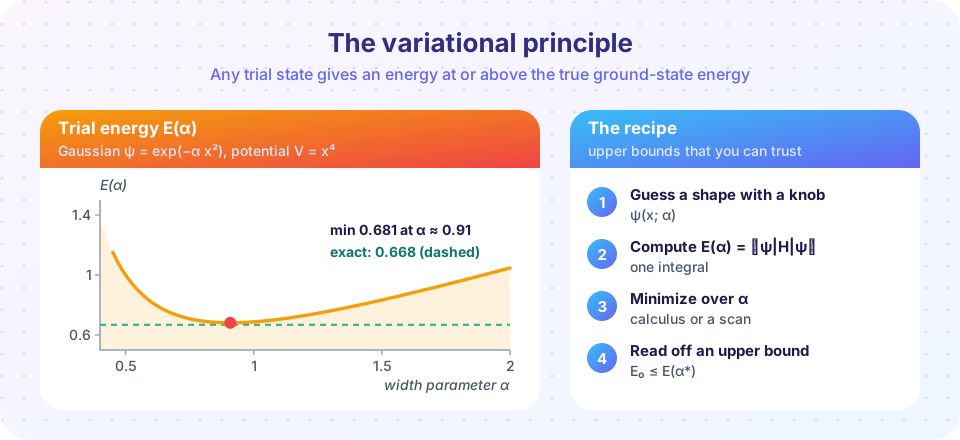
Take H = −½ d²/dx² + x⁴ (natural units), which cannot be solved in closed form. Try ψ = exp(−αx²). The standard Gaussian integrals give
⟨T⟩ = α/2, ⟨x⁴⟩ = 3/(16 α²) → E(α) = α/2 + 3/(16 α²)
Setting dE/dα = ½ − 3/(8α³) = 0 gives α³ = 3/4, α ≈ 0.9086, and E ≈ 0.6814. The accurate answer from a matrix calculation (last lesson) is about 0.6680, so one parameter lands within about 2 percent.
Example 2: hydrogen in atomic units
For hydrogen, H = −½∇² − 1/r, the exact ground state is exp(−r) with E = −1/2. Suppose we did not know that and tried a Gaussian exp(−αr²) instead. Integrals in three dimensions give
E(α) = 3α/2 − 2·√(2α/π)
with a minimum at α = 8/(9π) ≈ 0.283 and E = −4/(3π) ≈ −0.4244. That is above the exact −0.5, as it must be, but only about 15 percent off, because a Gaussian has the wrong shape at the nucleus (no cusp) and decays too fast far away. The bound E ≥ −0.5 is respected; the shape of the guess limits the quality.
Example 3: Monte Carlo and the local energy
For harder problems we cannot integrate. Instead we draw positions from |ψ|² (Metropolis algorithm) and average the local energy E_L = Hψ/ψ. For the oscillator H = −½d²/dx² + ½x² with the trial ψ = exp(−αx²):
E_L(x) = α + x² (½ − 2α²)
At α = ½ (the exact ground state) the x² term vanishes: E_L = ½ for every sample and the variance of the estimate is zero. This zero-variance property is a bonus: the closer your guess is to an eigenstate, the less noisy the Monte Carlo average becomes.
Common misconceptions
- "The variational energy is the average of the true levels." It is a weighted average over all eigenstates in your trial state, and weights favor the ground state when the guess is good.
- "If the trial energy is close to a known value, the wave function is accurate too." The energy error is second order in the wave-function error, so a decent energy can hide a poor shape (look at hydrogen's cusp).
- "More parameters can never hurt." They cannot raise the minimum energy, but the optimization becomes harder and can get stuck.
- "The method gives excited states." Only the lowest state of each symmetry, unless the trial is built to be orthogonal to lower states.
Try it
We check the analytic formula for E(α) by integrating numerically, scan α for the minimum, and compare with the matrix result from the last lesson.
Press Run (or Ctrl + Enter) to see the result here.
Program input · what you'd type while the program runs
Type the answers before you press Run, one per line. Each time the program reads a line (with input()), it gets the next line from this box.
Next, hydrogen. We evaluate the energy of an exponential and of a Gaussian trial function by numerical integration in 3D (radial integrals), and compare them with the formulas.
Press Run (or Ctrl + Enter) to see the result here.
Program input · what you'd type while the program runs
Type the answers before you press Run, one per line. Each time the program reads a line (with input()), it gets the next line from this box.
Finally, variational Monte Carlo for the harmonic oscillator. We sample positions from |ψ|² with a Metropolis walk and average the local energy. At α = 1/2 every sample gives exactly 1/2.
Press Run (or Ctrl + Enter) to see the result here.
Program input · what you'd type while the program runs
Type the answers before you press Run, one per line. Each time the program reads a line (with input()), it gets the next line from this box.
Check your understanding
Quick check · 5 questions
of 5 answered You scored / 5 · perfect!
-
1. The variational principle states that for any normalized trial state ψ...
⟨H⟩ is a weighted average of eigenvalues, all of which are at least E₀. -
2. A trial energy of -0.4244 is found for hydrogen (exact -0.5). What does this tell you?
A variational result is always at or above the exact energy, so -0.4244 > -0.5 is correct. -
3. For the quartic oscillator with ψ = exp(−αx²), the best α satisfies...
dE/dα = ½ − 3/(8α³) = 0 gives α³ = 3/4. -
4. The local energy is constant for...
If Hψ = Eψ then Hψ/ψ = E everywhere. -
5. Why does a better trial state give less noisy Monte Carlo energies?
Closer to an eigenstate means E_L is closer to constant, so its variance falls.
Summary
E(α) = ⟨ψ_α|H|ψ_α⟩/⟨ψ_α|ψ_α⟩ ≥ E₀: minimize over the parameters for the best bound.- Quartic oscillator:
E(α) = α/2 + 3/(16α²), minimum 0.681 against exact 0.668. Hydrogen with a Gaussian: −0.424 against −0.5. - The energy error is second order in the shape error, so check the wave function too.
- Monte Carlo averages the local energy
E_L = Hψ/ψover samples from|ψ|²; its variance vanishes for an exact eigenstate.
Next: Chapter 7 review
Track your progress
Create a free account to tick off lessons and pick up where you left off on any device.
of Computational Physics lessons completed