


















Lesson 24 of 47 · Partial Differential Equations
The heat equation and the FTCS scheme
Solve the 1D heat equation on a grid with the explicit FTCS scheme, see why r must stay below one half, and fix it with an implicit method.
Touch one end of a metal rod with a flame and the heat does not stay put: it spreads, and the sharp temperature difference smooths out. Joseph Fourier wrote the equation for this in 1822. It is the simplest PDE with time in it, which makes it the perfect first solver. You will march the temperature forward in small time steps, check your answer against an exact solution, and then discover what happens when the time step is too greedy.
What you will learn
- How to write the 1D heat equation and its boundary conditions.
- How the FTCS scheme derives from two finite differences.
- Why
r = αΔt/Δx²must be at most 1/2 for the explicit scheme. - How an implicit scheme (Crank-Nicolson) removes that limit.
Key terms
Thermal diffusivity (α): how fast temperature evens out, in m²/s. Copper is about 1.1e-4 m²/s, water about 1.4e-7 m²/s.
FTCS: Forward in Time, Centred in Space.
Dirichlet condition: the value at the boundary is fixed (for example, the ends kept at 0 degrees).
Courant-type number r: the dimensionless combination αΔt/Δx².
Implicit scheme: new values appear on both sides of the update, so a linear system must be solved each step.
The equation
For a thin rod with temperature u(x, t):
∂u/∂t = α · ∂²u/∂x²
The right side says: where the curve is bent upward (positive second derivative) the temperature rises, where it bends downward it falls. Peaks lose heat, valleys gain it.
Deriving FTCS
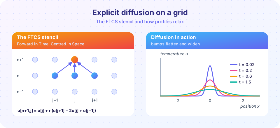
Approximate the time derivative with a forward difference and the space derivative with a central difference. Writing u[n, j] for the value at time step n and grid point j:
(u[n+1,j] − u[n,j]) / Δt = α (u[n,j+1] − 2u[n,j] + u[n,j−1]) / Δx²
Solve for the unknown new value:
u[n+1,j] = u[n,j] + r · (u[n,j+1] − 2u[n,j] + u[n,j−1]), r = α·Δt / Δx²
That is exactly the stencil in the picture. In NumPy the whole update is one line using slices, so no Python loop over space is needed.
A test with a known answer
On 0 ≤ x ≤ 1 with u = 0 at both ends and the starting profile sin(πx), the exact solution is exp(−π²αt) · sin(πx). The shape never changes, it just shrinks. A numerical solver that cannot reproduce this has a bug.
The stability limit
Why does r matter? Imagine a tiny zig-zag error: values alternating +ε, −ε. The FTCS update multiplies that zig-zag by 1 − 4r each step. If r > 1/2, then |1 − 4r| > 1 and the error doubles, then doubles again. This is not roundoff in a mysterious sense; it is a property of the scheme. For r ≤ 1/2 it stays bounded.
The limit has an expensive consequence. Halve Δx to get four times the spatial accuracy and you must cut Δt by four, so the total work grows by a factor of eight.
Common misconceptions
- "If the plot looks smooth, the scheme is stable." Instability often starts invisibly at the grid scale and takes a few dozen steps to explode.
- "A smaller Δx is always better." Without shrinking Δt as well, a smaller Δx pushes r above 1/2 and makes things worse.
- "Stable means accurate." A stable run can still be wrong if the grid is too coarse.
Implicit methods
The backward-in-time version evaluates the space difference at the new time. It is stable for every r, but each step needs a tridiagonal solve. The Crank-Nicolson scheme averages the old and new space differences, which is stable for all r and second-order accurate in time too. It is the standard choice for diffusion problems when you want long time steps.
Try it
First, the explicit solver against the exact solution. Everything is vectorized.
Press Run (or Ctrl + Enter) to see the result here.
Program input · what you'd type while the program runs
Type the answers before you press Run, one per line. Each time the program reads a line (with input()), it gets the next line from this box.
Now the stability experiment. The same code runs with r = 0.4 and r = 0.6; we print the largest absolute value after 100 steps.
Press Run (or Ctrl + Enter) to see the result here.
Program input · what you'd type while the program runs
Type the answers before you press Run, one per line. Each time the program reads a line (with input()), it gets the next line from this box.
Finally, an implicit Crank-Nicolson step with a huge r = 5, where FTCS would blow up instantly. We solve the tridiagonal system with a dense solver, which is fine for 41 points.
Press Run (or Ctrl + Enter) to see the result here.
Program input · what you'd type while the program runs
Type the answers before you press Run, one per line. Each time the program reads a line (with input()), it gets the next line from this box.
Check your understanding
Quick check · 5 questions
of 5 answered You scored / 5 · perfect!
-
1. In the FTCS scheme for the heat equation, which condition keeps it stable?
The explicit scheme multiplies a grid-scale error by 1 − 4r each step, so it is stable only when r is at most 1/2. -
2. You halve Δx to improve spatial accuracy and keep r at 0.4. By what factor does Δt change?
Δt = rΔx²/α, so halving Δx divides Δt by four. -
3. What is the main price of an implicit method such as Crank-Nicolson?
Implicit methods couple all new values together, so each step requires solving a (tridiagonal) linear system. -
4. The exact solution sin(πx)·exp(−π²αt) shows that the temperature profile...
The sine is an eigenfunction of the second derivative, so only its amplitude decays. -
5. A thermal diffusivity of 1.1e-4 m²/s (copper) versus 1.4e-7 m²/s (water) means heat...
A larger α means faster smoothing of temperature differences.
Summary
- The heat equation
u_t = α·u_xxsmooths temperature profiles; its exact test case is a decaying sine. - FTCS:
u_new = u + r·(u[j+1] − 2u + u[j−1])withr = αΔt/Δx². - Stability needs
r ≤ 1/2; refining the grid forces much smaller time steps. - Implicit schemes such as Crank-Nicolson remove the limit at the cost of a linear solve per step.
Track your progress
Create a free account to tick off lessons and pick up where you left off on any device.
of Computational Physics lessons completed