


















Lesson 31 of 47 · Molecular Dynamics
Temperature, pressure and structure
Turn raw trajectories into physics: kinetic temperature, virial pressure, velocity-rescaling thermostat and the radial distribution function of a Lennard-Jones liquid.
An MD run produces millions of numbers: positions and velocities of every atom at every step. Nobody reads that. The art is in turning raw trajectories into a few meaningful quantities. In this lesson you will measure the three most common ones: temperature (from motion), pressure (from forces and motion) and the radial distribution function (from structure). You will also learn how to bring a simulation to a target temperature.
What you will learn
- How kinetic energy gives the temperature and why we divide by the degrees of freedom.
- How the virial expression gives the pressure.
- What the radial distribution function measures and how to compute it.
- How a velocity-rescaling thermostat works, and its limits.
Key terms
Equipartition theorem: in equilibrium each quadratic degree of freedom carries on average ½ k_B T of energy.
Degrees of freedom (N_f): independent motions. For N atoms in d dimensions with fixed total momentum, N_f = d(N − 1).
Virial: the sum Σ r_ij · F_ij over pairs, a measure of how strongly the atoms push and pull.
Radial distribution function g(r): the density of atoms at distance r from a typical atom, divided by the average density.
Thermostat: a trick that keeps the temperature near a target value.
Temperature
The equipartition theorem says each degree of freedom has mean kinetic energy ½ k_B T. In reduced units (k_B = m = 1):
T = (Σ v_i²) / (d · N_f) with N_f = N − 1 (one fewer because the total momentum is fixed)
An instantaneous temperature fluctuates from step to step; the average over a long run is the meaningful number. The relative fluctuation shrinks like 1/√N, so small systems have noisy temperatures.
Pressure
Pressure has two parts: the ideal-gas term (atoms hitting the walls) and a correction from interactions. For pair forces in a periodic box of volume V (area in 2D):
P = ρ T + (1 / (d V)) · Σ_{i<j} r_ij · F_ij
When atoms mostly repel each other the second term is positive (pressure raised); when they attract, negative (pressure lowered). That is why a dense, compressed liquid has a large pressure and a stretched one can have negative pressure.
The radial distribution function
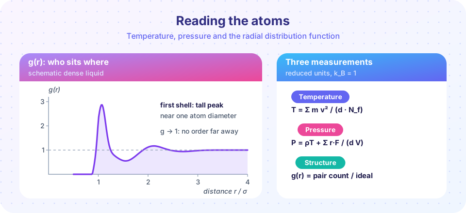
Imagine sitting on one atom and counting its neighbors in rings of increasing radius. In a dilute gas, the count in a ring grows with the ring's area (2D) or volume (3D). The function g(r) is the actual count divided by what an ideal gas of the same density would give:
g(r) = (number of pairs in the shell [r, r+dr]) / (N·ρ·shell_volume / 2)
(the factor 1/2 because each pair is counted once). What it looks like:
g = 0forr < σ: atoms cannot overlap.- A tall peak near
r ≈ σ: the first shell of touching neighbors. - A dip, then smaller peaks: layers of shells.
g → 1at larger: far from the central atom, density is average.
In a crystal the peaks are sharp and persist; in a gas there is almost no structure. Real g(r) curves can be measured by X-ray and neutron scattering, which makes this the key link between a simulation and an experiment. Remember to stop at r = L/2, the largest distance for which minimum-image distances are meaningful.
Thermostats
Left alone, the simulation conserves energy: microcanonical (NVE) ensemble. To simulate at a fixed temperature (NVT) you couple the atoms to a heat bath. The simplest method rescales all velocities by √(T_target / T_now). This is fine for the equilibration phase (getting rid of the artificial starting configuration) but does not generate the correct fluctuations. For production runs, researchers use the Nosé-Hoover thermostat or the Langevin approach, which are built on solid statistical mechanics. A very common recipe: equilibrate with rescaling, then switch to NVE and measure.
Common misconceptions
- "Temperature is a property of a single atom." It is a statistical property of many atoms; one velocity says nothing.
- "Start measuring from step 1." The first stretch of the run still remembers the artificial starting grid. Discard it as equilibration.
- "The g(r) peak height is the number of neighbors." The number of neighbors is the integral of
ρ g(r)over the first shell, not the height. - "Rescaling velocities at every step is a proper thermostat." It removes the natural temperature fluctuations.
Try it
A complete two-dimensional Lennard-Jones simulation: 100 atoms at reduced density 0.8 and temperature 1. It melts the initial square lattice, equilibrates with rescaling, then measures temperature, pressure and g(r). The run takes a few seconds.
Press Run (or Ctrl + Enter) to see the result here.
Program input · what you'd type while the program runs
Type the answers before you press Run, one per line. Each time the program reads a line (with input()), it gets the next line from this box.
The next example shows why a thermostat is needed. Starting with all atoms on a lattice, the potential energy turns into kinetic energy and the temperature changes without any thermostat. We print the temperature during an NVE run.
Press Run (or Ctrl + Enter) to see the result here.
Program input · what you'd type while the program runs
Type the answers before you press Run, one per line. Each time the program reads a line (with input()), it gets the next line from this box.
The temperature moves away from the initial 1.0 because kinetic and potential energy trade places during melting. This is normal: only the sum is conserved.
Check your understanding
Quick check · 5 questions
of 5 answered You scored / 5 · perfect!
-
1. For N atoms in 3 dimensions with fixed total momentum, how many degrees of freedom enter the temperature?
Fixing the total momentum removes 3 degrees of freedom, so N_f = 3(N − 1). -
2. In a dense liquid, g(r) at r much larger than σ approaches...
Far from a given atom the density is the average density, so the ratio is 1. -
3. Strong repulsion between atoms makes the interaction part of the pressure...
Repulsive forces push atoms apart, so r·F is positive and raises the pressure. -
4. Why is velocity rescaling at every step not a proper thermostat for production runs?
A canonical ensemble has fluctuating kinetic energy; rescaling forces it to be constant. -
5. Why do we only compute g(r) up to L/2?
With minimum image distances nothing is farther than about L/2 along each axis, and shells beyond it are incomplete.
Summary
T = Σ v² / (d·N_f)in reduced units, withN_f = d(N − 1); average over many steps.P = ρT + Σ r·F / (dV): a kinetic part plus an interaction (virial) part.g(r)counts pairs in shells relative to an ideal gas: zero inside σ, a tall first peak, decaying toward 1.- Equilibrate (rescale velocities), then measure without interference; use a proper thermostat for NVT production runs.
Next: Chapter 6 review
Track your progress
Create a free account to tick off lessons and pick up where you left off on any device.
of Computational Physics lessons completed