


















Lesson 17 of 47 · Monte Carlo Methods
Monte Carlo Methods: Overview
Preview chapter 4: how random sampling solves problems in physics, from estimating pi to random walks and the Ising model, and why the error falls as one over the square root of N.
Time stepping follows one trajectory carefully. Monte Carlo methods do something different: they use random numbers to sample many possibilities and read the answer from averages. The idea is old and strangely powerful. To find the area of a lake, throw a thousand stones at random into a rectangle that contains it and count how many splash. To find the pressure of a gas, sample typical configurations of its molecules and average. Randomness replaces a computation that would be impossibly large.
What you will learn
- Where Monte Carlo came from and what problems it suits.
- The core principle: estimate an average by sampling.
- The
1/√Nerror law and what it implies. - What each lesson in this chapter covers.
Key terms
Monte Carlo method: any computation that uses random sampling to estimate a quantity.
Pseudo-random numbers: numbers from a deterministic algorithm that behave like random ones.
Sample: one randomly generated configuration or value.
Statistical error: the uncertainty of an estimate caused by finite sampling; it falls like 1/√N.
The idea
When it shines
In this chapter
A short history
The method was born at Los Alamos in the 1940s. Stanislaw Ulam, recovering from an illness, wondered about the chance of winning solitaire and realized that playing many random games and counting wins would be easier than combinatorics. With John von Neumann and Nicholas Metropolis he applied the idea to neutron diffusion in nuclear weapons research, using the first electronic computers. The code name "Monte Carlo" referred to the casino. In 1953, Metropolis, the Rosenbluths and the Tellers published an algorithm for sampling the states of a thermal system, the ancestor of the Metropolis method you will meet in the Ising lesson.
The core principle
Suppose you want the average ⟨f⟩ of some quantity over a distribution of states. If you can draw N independent samples x₁ … x_N from the distribution, then
⟨f⟩ ≈ (1/N) Σ f(xᵢ)
and the statistical error is about σ/√N, where σ is the standard deviation of f. Two facts matter:
- The error does not depend on the dimension. A grid-based integral in 10 dimensions with just 10 points per axis needs
10¹⁰evaluations. A Monte Carlo estimate with10⁶samples has the same1/√Nerror for 1 or 100 dimensions. - The convergence is slow. To gain one more digit of accuracy you need 100 times more samples. Cleverness (variance reduction) matters more than raw speed.
Your first estimate: darts and pi
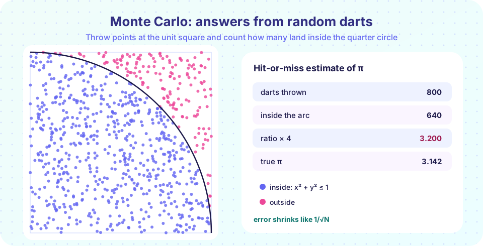
Throw N points uniformly into the unit square [0, 1] × [0, 1]. The fraction landing inside the quarter circle x² + y² ≤ 1 is the ratio of areas, (π/4)/1. So π ≈ 4 × (hits / N).
Press Run (or Ctrl + Enter) to see the result here.
Program input · what you'd type while the program runs
Type the answers before you press Run, one per line. Each time the program reads a line (with input()), it gets the next line from this box.
The error shrinks, but not smoothly: each run is a random draw. A seed (default_rng(2024)) makes the experiment repeatable.
The statistics of the estimate
Each dart is a Bernoulli trial: it hits with probability p = π/4 ≈ 0.785. The number of hits has variance N p (1 − p), so the standard error of 4 hits / N is
4 √(p(1 − p) / N) ≈ 1.64 / √N
For N = 10⁶ that is about 0.0016. You can predict the typical error in advance. This is the key habit of Monte Carlo: always report the estimate together with its statistical error.
Press Run (or Ctrl + Enter) to see the result here.
Program input · what you'd type while the program runs
Type the answers before you press Run, one per line. Each time the program reads a line (with input()), it gets the next line from this box.
Map of the chapter
- Random Numbers and Sampling: how computers make random numbers and how to turn uniform numbers into any distribution.
- Monte Carlo Integration: averaging a function, the
1/√Nlaw and variance reduction. - Random Walks and Diffusion: steps in space, the link to diffusion.
- The Ising Model and Metropolis: sampling thermal states of a magnet.
- Chapter 4 Review: recap and quiz.
Common misconceptions
"A bigger N makes the error go to zero quickly." It falls only as 1/√N: a hundred times more samples for one more digit.
"Pseudo-random numbers are not random enough for physics." Modern generators pass stringent statistical tests. The danger is poor old generators and unseeded or reused streams.
"One run is enough." A single run gives a single number. Without an error estimate you cannot say whether it is good.
Check your understanding
Quick check · 4 questions
of 4 answered You scored / 4 · perfect!
-
1. How does the statistical error of a Monte Carlo average scale with the number of samples N?
The standard error is sigma divided by the square root of N. -
2. You want ten times smaller error. How many more samples?
Error falls like 1/sqrt(N), so a tenfold gain needs 100 times more samples. -
3. Why is Monte Carlo attractive in high dimensions?
Grid methods need exponentially many points; the Monte Carlo error depends on N and the variance, not the dimension. -
4. In the darts estimate, what does the ratio hits / N approximate?
The quarter circle has area pi/4 inside a unit square of area 1.
Summary
- Monte Carlo estimates averages from random samples; the error falls like
1/√N. - The scaling is independent of dimension, which is why it handles problems that grids cannot.
- Always report an estimate with its statistical error and seed your generator.
- The next lesson shows how random numbers are made and shaped.
Track your progress
Create a free account to tick off lessons and pick up where you left off on any device.
of Computational Physics lessons completed