


















Lesson 39 of 47 · Data Analysis and Projects
Fitting models to data
Fit lines and curves to data with weighted least squares, read parameter uncertainties from chi-square and covariance, and compare with a bootstrap.
You measure the period of a pendulum for ten different lengths, or record the temperature of a simulated liquid at ten densities. A theory predicts the points should lie on a curve with a few unknown numbers in it. Your task is to find the numbers and to say how well you know them. This is fitting, and almost every physics result you read comes from one.
What you will learn
- What least squares minimizes and why points are weighted by
1/σ². - How to compute slope, intercept and their uncertainties for a line.
- How to fit a nonlinear model with
scipy.optimize.curve_fitand read the covariance matrix. - How to judge a fit with
χ²/dofand residuals, and how the bootstrap checks the error bars.
Key terms
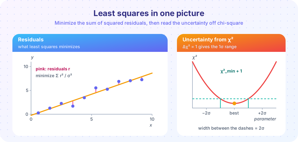
Least squares: choose the parameters that minimize χ² = Σ ((y_i − f(x_i)) / σ_i)².
Degrees of freedom (dof): number of data points minus number of fitted parameters.
Reduced chi-square: χ²/dof; about 1 for a good fit with correct error bars.
Covariance matrix: its diagonal holds the squared parameter uncertainties; off-diagonal entries show how parameters trade off.
Bootstrap: re-sample your data with replacement many times, refit each time, and use the spread of results as the uncertainty.
What is being minimized
Given points (x_i, y_i) with uncertainties σ_i and a model f(x; p) with parameters p, define
χ²(p) = Σ_i ( (y_i − f(x_i; p)) / σ_i )²
Each term is the squared miss of one point measured in units of its own uncertainty. A point with a small σ is trusted more and pulls the curve harder. If the noise is Gaussian, minimizing χ² gives the most probable parameters (maximum likelihood). Legendre and Gauss introduced the method around 1800 to fit planetary orbits to observations.
A straight line, by formula
For y = m x + b define S = Σ 1/σ², S_x = Σ x/σ², S_y = Σ y/σ², S_xx = Σ x²/σ², S_xy = Σ xy/σ², and Δ = S·S_xx − S_x². Then
m = (S·S_xy − S_x·S_y) / Δ,     b = (S_xx·S_y − S_x·S_xy) / Δ
σ_m² = S / Δ,                    σ_b² = S_xx / Δ
The formulas look heavy but are just a few sums, so they are easy to code and to check against a library.
Uncertainty from the shape of χ²
Near its minimum, χ² is a parabola in each parameter: χ²(p) ≈ χ²_min + ((p − p̂)/σ_p)². The parameter has risen by exactly one standard deviation when χ² has gone up by 1. So "scan the parameter, find where χ² increases by 1" is a direct way to get the 1σ interval, and it works even when the parabola is lopsided (nonlinear fits).
Is the fit any good?
χ²/dof ≈ 1: the model agrees with the data within the stated errors.χ²/dof ≫ 1: the model is wrong, or the error bars are too small, or there are outliers.χ²/dof ≪ 1: the error bars are probably too large (or the data were tuned).- Look at residuals: a good fit leaves a cloud of points with no pattern. A trend or wave in the residuals shows a missing term in the model, even when
χ²/doflooks fine.
Common misconceptions
- "A high R² proves the model is right." A wrong model can have an R² of 0.99. Check residuals and
χ²/dof. - "The fitted parameter has no uncertainty if the curve passes through all points." More parameters than needed can pass through all points and still be meaningless.
- "Error bars from
curve_fitare always absolute." By defaultcurve_fitrescales the covariance by the observed scatter. Passabsolute_sigma=Truewhen yourσ_iare real measurement errors. - "Fit the logarithm to get an exponential." It can work, but it changes the weights; fit the original data when you can.
Try it
Everything below uses synthetic data: points generated from a known line plus noise, so we can check whether the fit recovers the truth. First the formulas against numpy and a plot with a 1σ band.
Press Run (or Ctrl + Enter) to see the result here.
Program input · what you'd type while the program runs
Type the answers before you press Run, one per line. Each time the program reads a line (with input()), it gets the next line from this box.
Now a nonlinear model. A radioactive sample is counted for 1 time unit at a series of times; the counts are Poisson distributed with mean N₀·exp(−λt), and the uncertainty of each count is about √N. We fit with curve_fit and check χ²/dof.
Press Run (or Ctrl + Enter) to see the result here.
Program input · what you'd type while the program runs
Type the answers before you press Run, one per line. Each time the program reads a line (with input()), it gets the next line from this box.
Finally, two independent checks of the slope's uncertainty for the first data set: the Δχ² = 1 rule and a bootstrap that resamples the points.
Press Run (or Ctrl + Enter) to see the result here.
Program input · what you'd type while the program runs
Type the answers before you press Run, one per line. Each time the program reads a line (with input()), it gets the next line from this box.
The bootstrap result is usually a little larger than the formula for small samples, because resampled data sets sometimes cluster their x values and lose leverage. For 10 points the two methods agree roughly; for 1000 points they agree very well.
Check your understanding
Quick check · 5 questions
of 5 answered You scored / 5 · perfect!
-
1. In weighted least squares, a point with a small uncertainty σ...
Each residual is divided by σ, so precise points contribute more to χ² and to the fit. -
2. A fit has 12 points, 2 parameters and χ² = 9.6. What is χ²/dof?
dof = 12 − 2 = 10, so χ²/dof = 0.96, consistent with a good fit. -
3. How do you get a 1σ parameter uncertainty from a χ² scan?
Δχ² = 1 marks one standard deviation for Gaussian errors. -
4. The residuals show a clear sine-like wave. What does this indicate?
Residuals should be random. A pattern means the model leaves out something. -
5. Why pass absolute_sigma=True to curve_fit?
Without it, SciPy rescales the covariance so that χ²/dof = 1, which hides a bad model.
Summary
- Least squares minimizes
χ² = Σ((y − f)/σ)²; weights1/σ²trust precise points more. - A weighted line fit has closed formulas for
m,b,σ_m,σ_b;curve_fithandles any model. χ²/dof ≈ 1and structureless residuals indicate a good fit; useabsolute_sigma=Truefor true error bars.- Uncertainties can be checked three ways: covariance matrix, the
Δχ² = 1rule and the bootstrap.
Track your progress
Create a free account to tick off lessons and pick up where you left off on any device.
of Computational Physics lessons completed