


















Lesson 23 of 47 · Partial Differential Equations
Chapter overview: partial differential equations
See the big picture of numerical PDEs: heat, wave and Laplace equations, why grids work, and what every lesson in this chapter covers.
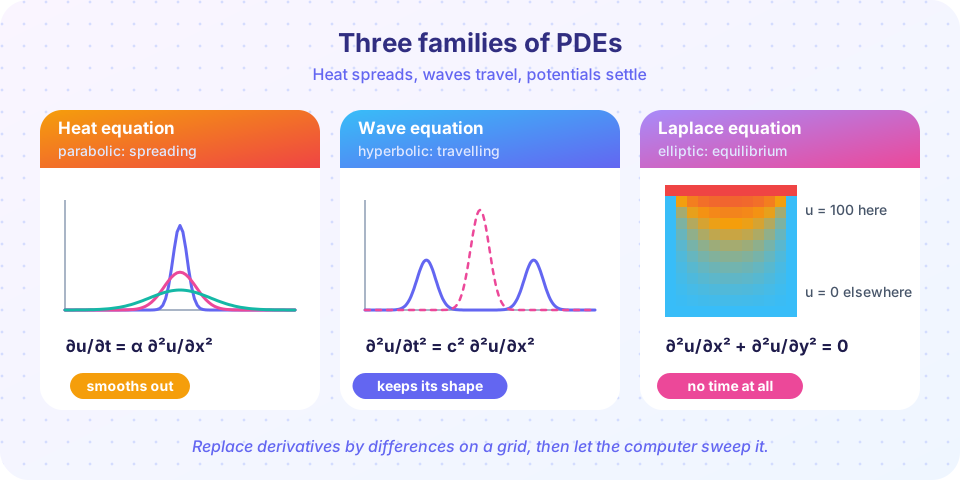
Most of physics is written in partial differential equations (PDEs). Heat flows through a metal bar, a guitar string vibrates, an electric potential settles around a charged plate: each of these involves a quantity that depends on several variables at once, such as position and time. Only a few PDEs have neat pencil-and-paper solutions. For everything else, you teach the computer to approximate the answer on a grid.
This chapter builds that skill with the three classic model equations. If you can simulate these three, you can read and adapt almost any PDE solver you meet later.
What you will learn
- Why a PDE is turned into a set of ordinary arithmetic steps on a grid.
- How the heat, wave and Laplace equations differ in behavior and in the numerical method they need.
- What stability, accuracy and convergence mean in practice.
- What each of the next four lessons teaches.
Key terms
Partial derivative: the rate of change of a quantity with respect to one variable while the others are held fixed.
Grid (mesh): a set of points in space and time where we store approximate values.
Finite difference: a formula that replaces a derivative by a difference of grid values.
Boundary condition: the value (or slope) the solution must have at the edge of the region.
Stability: small errors stay small instead of growing step after step.
The big idea: derivatives become differences
A second derivative at a grid point is estimated from its neighbors:
∂²u/∂x² ≈ (u[j+1] − 2·u[j] + u[j−1]) / Δx²
Do the same for time and each PDE turns into a rule that says "the new value at this point is a combination of old values nearby". The computer then applies the rule millions of times. The error of this central difference shrinks like Δx²: halve the spacing and the error drops by a factor of about four.
Three behaviors, three methods
Heat equation
Wave equation
Laplace equation
The workflow
Mathematicians call the three families parabolic (heat), hyperbolic (wave) and elliptic (Laplace). The names matter for one practical reason: they tell you how information moves. In a parabolic problem it spreads out everywhere instantly but weakly. In a hyperbolic problem it moves at a finite speed. In an elliptic problem every point depends on the whole boundary at once, so you solve for all points together.
What each lesson covers
- The heat equation and the FTCS scheme: your first solver, a stability experiment, and the implicit fix.
- The wave equation and the leapfrog scheme: vibrating strings, the CFL condition and numerical dispersion.
- The Laplace equation and relaxation: Jacobi, Gauss-Seidel and SOR, with iteration counts.
- Chapter 5 review: a one-page picture and a ten-question quiz.
Try it
A PDE of the form A·u_xx + B·u_xy + C·u_yy + … = 0 is classified by the sign of B² − 4AC. The tool below applies that rule. It is a calculator for the classification only, not a solver.
Press Run (or Ctrl + Enter) to see the result here.
Program input · what you'd type while the program runs
Type the answers before you press Run, one per line. Each time the program reads a line (with input()), it gets the next line from this box.
A second experiment: how fast does the central-difference error shrink? We estimate the second derivative of sin(x) at x = 1 (exact value −sin 1).
Press Run (or Ctrl + Enter) to see the result here.
Program input · what you'd type while the program runs
Type the answers before you press Run, one per line. Each time the program reads a line (with input()), it gets the next line from this box.
Each time dx is halved the error falls by about a factor of four: second-order accuracy.
Check your understanding
Quick check · 4 questions
of 4 answered You scored / 4 · perfect!
-
1. Which PDE describes a steady state with no time variable?
The Laplace equation has only space variables. Its solution is the state that remains once everything has settled. -
2. What does a finite difference do?
A finite difference approximates a derivative using values at neighboring grid points. -
3. If a second-order scheme has spacing 0.1 and error 4e-4, roughly what error do you expect at spacing 0.05?
Second order means error scales with dx squared. Halving dx divides the error by 4. -
4. In which type of PDE does information travel at a finite speed?
Hyperbolic equations such as the wave equation carry disturbances at a finite speed.
Summary
- A PDE is solved numerically by storing values on a grid and replacing derivatives with differences.
- Heat (parabolic) spreads, wave (hyperbolic) travels, Laplace (elliptic) describes balance.
- Each type needs its own method and its own stability rule.
- Always test a new solver on a case with a known exact answer.
Track your progress
Create a free account to tick off lessons and pick up where you left off on any device.
of Computational Physics lessons completed