


















Lesson 22 of 47 · Monte Carlo Methods
Chapter 4 Review: Monte Carlo Methods
Review chapter 4: random numbers and sampling, Monte Carlo integration, random walks and the Metropolis algorithm for the Ising model, with a recap table and a ten-question quiz.
Chapter 4 introduced a new way of computing: instead of following one path precisely, sample many paths randomly and average. You made random numbers, shaped them into physical distributions, estimated integrals with error bars, watched diffusion emerge from random steps and found a phase transition with Metropolis sampling. This review ties the pieces together.
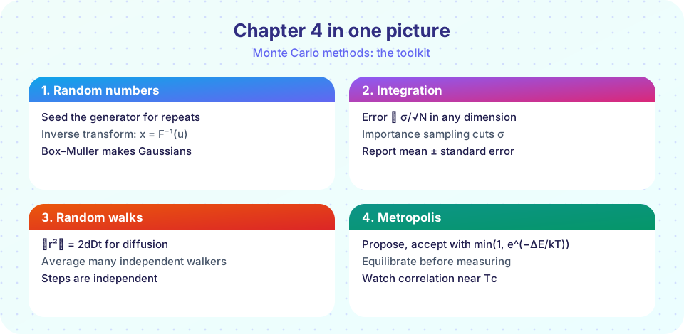
What you will review
- Seeds, PRNGs and the three sampling recipes.
- The sample mean, standard error and the
1/√Nlaw. - Random walks, MSD and the diffusion coefficient.
- Metropolis sampling and the Ising transition.
Recap table
| Topic | Key formula | Check |
|---|---|---|
| Overview | π ≈ 4 · hits / N, error ∝ 1/√N |
Does the error shrink 10× for 100× more samples? |
| Sampling | t = −τ ln(1 − u), Box-Muller, rejection |
Histogram and known moments match? |
| Integration | Î = (b−a) mean(f), SE = σ̂/√N |
Is the estimate within a few SE of a known answer? |
| Random walks | ⟨r²⟩ = 2 d D t |
Is the MSD a straight line in time? |
| Ising model | P(accept) = min(1, e^(−ΔE/kT)), Tc = 2.269 |
Does ` |
One toolkit, four problems
The code below packages the pattern used throughout the chapter: draw samples, compute a mean and a standard error, compare with the exact answer. It applies to a ball-in-a-square problem, an exponential lifetime probability, a Gaussian moment, and an integral with importance sampling.
Press Run (or Ctrl + Enter) to see the result here.
Program input · what you'd type while the program runs
Type the answers before you press Run, one per line. Each time the program reads a line (with input()), it gets the next line from this box.
Every estimate lies within a few standard errors of the exact value. If one did not, you would suspect a bug or a biased sampler, exactly the kind of check this chapter has encouraged.
Habits that pay off
- Seed and record.
default_rng(seed)and write the seed down. - Attach an error bar. A Monte Carlo number without an uncertainty is not a result.
- Test on a known case. Run the sampler on a problem with an exact answer first.
- Equilibrate. For Markov-chain methods such as Metropolis, discard burn-in and watch for slow correlations.
- Vectorize. One NumPy operation over all walkers or all spins beats a Python loop.
Chapter review quiz
Quick check · 10 questions
of 10 answered You scored / 10 · perfect!
-
1. By what factor must N grow to cut the statistical error of a Monte Carlo average by 5?
Error is proportional to 1/sqrt(N), so a factor 5 needs 25 times more samples. -
2. To sample the exponential density with mean tau by inverse transform you compute
Invert the CDF F(t) = 1 - exp(-t / tau). -
3. Which recipe gives uniform random directions on a sphere?
Equal intervals of cos(theta) correspond to equal areas on the sphere. -
4. The standard error of a sample mean is estimated as
sigma_hat divided by the square root of N. -
5. After N unit steps of a 1D walk the typical distance is about
The MSD is N, so the rms distance is sqrt(N). -
6. For a 3D walk, <r^2> = 6 D t. If MSD = 12 after t = 4 s, D is
D = MSD / (6 t) = 12 / 24 = 0.5. -
7. In Metropolis sampling, a move that lowers the energy is
Only moves that raise the energy are accepted probabilistically. -
8. Why is burn-in discarded?
The Markov chain needs time to reach equilibrium. -
9. Importance sampling estimates an integral by averaging
The ratio corrects for sampling from p. -
10. Near the critical temperature of the Ising model, what happens to successive Metropolis samples?
Large fluctuating domains take many sweeps to change, so effective sample counts are smaller.
Summary
- Monte Carlo estimates averages from samples; the error is
σ/√Nin any dimension. - Inverse transform, Box-Muller and rejection turn uniforms into physical distributions.
- Random walks produce linear MSD and connect to diffusion; Metropolis samples thermal states.
- Seed, equilibrate, test on a known case and report errors.
- Chapters 5 to 7 move on to fields, atoms and quantum systems, building on everything so far.
Track your progress
Create a free account to tick off lessons and pick up where you left off on any device.
of Computational Physics lessons completed