


















Lesson 44 of 47 · Projects and Practice
Practice set: eight exercises
Eight hands-on exercises covering PDEs, molecular dynamics, quantum tunneling, fitting, spectra and convergence, with hints and self-checking Python solutions.
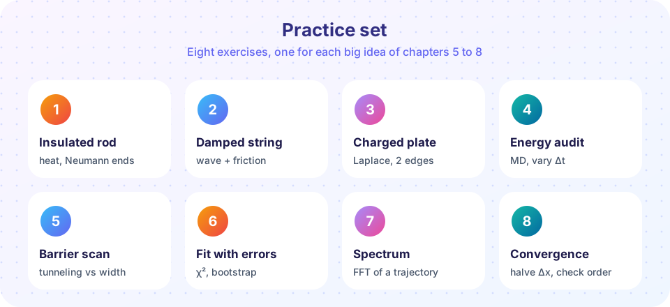
You learn numerical methods by breaking them, fixing them and checking them against something you know. This practice set gives you eight short exercises, one for each big idea of chapters 5 to 8. Each has a goal, a hint and a self-check: a number or a property that tells you whether you got it right. Try each exercise yourself first; solution code for four of them is in the editors below.
How to use this page
- Read the exercise and sketch the plan on paper.
- Write the code. Test the smallest piece first.
- Compare with the self-check. If it fails, look at the hint, then at the solution.
- Change one parameter and predict the result before running again.
The exercises
1. Insulated rod (heat, chapter 5). A rod with both ends insulated cannot lose heat, so the total heat must stay constant. Implement FTCS with zero-slope boundaries (u[0] = u[1], u[-1] = u[-2]) starting from a bump. Hint: update interior points first, then copy the neighbors to the ends. Self-check: the sum of u stays within a few percent of its start while the profile flattens to a constant. (Copying the neighbor is only a first-order boundary, so a small error remains; a ghost-point boundary would shrink it.)
2. Damped string (wave, chapter 5). Add friction to the wave equation: u_tt + γ u_t = c² u_xx. A standing wave sin(πx) should decay as exp(−γt/2) when γ is small. Hint: replace the time derivatives by central differences and solve for u[n+1]. Self-check: the measured decay rate matches γ/2.
3. Charged plate (Laplace, chapter 5). Two opposite edges of a square are held at +1 and −1, the other two edges at 0. Hint: the problem is antisymmetric, so the potential in the exact center must be 0. Self-check: center value 0 within the convergence tolerance.
4. Energy audit (molecular dynamics, chapter 6). Run a small Lennard-Jones box at Δt = 0.002, 0.004, 0.008, 0.016 and plot the energy fluctuation against Δt. Hint: reuse the code of the Verlet lesson and use a log-log plot. Self-check: slope of about 2.
5. Barrier scan (quantum, chapter 7). Compute the transmission through barriers of width 0.5, 1.0, 1.5 and 2.0 at fixed height 3 and wave-packet energy 2. Hint: make sure the width is a whole number of grid cells. Self-check: agreement with the exact T(E) formula to a few percent; T falls roughly exponentially with width.
6. Fit with errors (data, chapter 8). Synthetic pendulum data: lengths L with periods T that have an uncertainty of 0.01 s. Fit T² = (4π²/g) L and report g with its uncertainty. Self-check: the true value (9.81 m/s²) lies within about two uncertainties.
7. Spectrum of a trajectory (data, chapter 8). Simulate an anharmonic oscillator x'' = −x − εx³ and find the frequency of its motion from the FFT. Hint: use a Hann window and interpolate the peak position. Self-check: for ε = 0.2 and amplitude 1, first-order perturbation theory predicts ω ≈ 1 + 3εA²/8 = 1.075.
8. Convergence (all chapters). Solve the heat equation on Δx and Δx/2 (with the same r), compare with the exact solution and compute the observed order p = log₂(e₁/e₂). Self-check: p ≈ 2 in space.
Common misconceptions about practice
- "If the picture looks plausible, the code is right." Plausible pictures hide wrong factors of two. Always compare a number with a known value.
- "Copy the solution once and move on." Change a parameter and predict the outcome; that is where learning happens.
- "Convergence tests are only for papers." They are the cheapest way to find a bug in a solver.
Try it: solutions for exercises 1 and 2
The insulated rod keeps nearly all of its heat (the first-order boundary copy leaves a small error, so we print how much). The damped string measures its decay rate from the peak amplitude.
Press Run (or Ctrl + Enter) to see the result here.
Program input · what you'd type while the program runs
Type the answers before you press Run, one per line. Each time the program reads a line (with input()), it gets the next line from this box.
Try it: solutions for exercises 6 and 7
For the pendulum fit we generate synthetic data from g = 9.81 and fit the line T² against L. For the spectrum we integrate the anharmonic oscillator with velocity Verlet and locate the FFT peak by parabolic interpolation.
Press Run (or Ctrl + Enter) to see the result here.
Program input · what you'd type while the program runs
Type the answers before you press Run, one per line. Each time the program reads a line (with input()), it gets the next line from this box.
Try it: solution for exercise 8
Convergence of the explicit heat solver. We keep r = 0.4 fixed (so Δt shrinks four times when Δx halves) and compare each run with the exact solution at the same time.
Press Run (or Ctrl + Enter) to see the result here.
Program input · what you'd type while the program runs
Type the answers before you press Run, one per line. Each time the program reads a line (with input()), it gets the next line from this box.
Check your understanding
Quick check · 4 questions
of 4 answered You scored / 4 · perfect!
-
1. In exercise 1, why must the total heat be nearly constant?
With zero-flux boundaries, heat can only move around inside the rod. -
2. In exercise 6, if the fitted slope of T² against L is 4.02 s²/m, what is g?
g = 4π²/slope = 39.478/4.02 ≈ 9.82 m/s². -
3. In exercise 8 the observed order comes out near 2. What does this show?
If errors fall by 4 when Δx is halved, log₂(4) = 2 and the scheme is second order in space. -
4. Why interpolate the FFT peak in exercise 7?
The true peak lies between bins; interpolation recovers it more precisely than the resolution suggests.
Summary
- Each exercise has a self-check: a conserved total, a known frequency, a known value or an expected convergence order.
- Test small, compare numbers, then change one parameter and predict.
- Observed order
p = log₂(e₁/e₂)is the fastest way to find a bug in a solver.
Next: Glossary and units
Track your progress
Create a free account to tick off lessons and pick up where you left off on any device.
of Computational Physics lessons completed