


















Lesson 18 of 47 · Monte Carlo Methods
Random Numbers and Sampling
Learn how pseudo-random generators work, why seeds matter, and how to sample exponential, Gaussian and direction distributions by inverse transform, Box-Muller and rejection.
Every Monte Carlo program starts with a stream of random numbers, and almost every physics problem needs them shaped into a specific distribution: exponential lifetimes for radioactive decay, Gaussian velocities for a gas, uniform directions for a scattered neutron. This lesson shows where the numbers come from and the three standard recipes for turning uniform numbers into anything else.
What you will learn
- How a pseudo-random generator works and why seeds make runs repeatable.
- The inverse-transform method, with exponential lifetimes as an example.
- The Box-Muller transform for Gaussian numbers.
- Rejection sampling when the inverse is not available.
- How to pick random directions uniformly on a sphere.
Key terms
PRNG: a pseudo-random number generator, a deterministic algorithm with an internal state.
Seed: the initial state; the same seed gives the same stream.
CDF F(x): the probability that the variable is at most x.
PDF f(x): the probability density, f = dF/dx.
Uniform deviate u: a random number uniformly distributed in [0, 1).
Pseudo-random generators
A computer cannot toss a coin; it computes numbers that pass statistical tests of randomness. The classic example is the linear congruential generator (LCG):
x_{n+1} = (a x_n + c) mod m, u_n = x_n / m
With well chosen a, c, m the sequence looks random but repeats after at most m numbers (the period). Poor parameters give short periods and visible patterns; the infamous RANDU generator from the 1960s put triples of numbers on a small number of planes. NumPy's default generator, np.random.default_rng(), uses the PCG64 algorithm: a huge period (2¹²⁸) and excellent statistics. Always use it rather than the older global np.random.rand.
Press Run (or Ctrl + Enter) to see the result here.
Program input · what you'd type while the program runs
Type the answers before you press Run, one per line. Each time the program reads a line (with input()), it gets the next line from this box.
Seeds. default_rng(42) always returns the same stream, which makes bugs reproducible and published results checkable. For parallel runs use np.random.SeedSequence(42).spawn(k) to create k statistically independent child streams; never seed several workers with consecutive integers by hand and assume they are independent.
Inverse-transform sampling
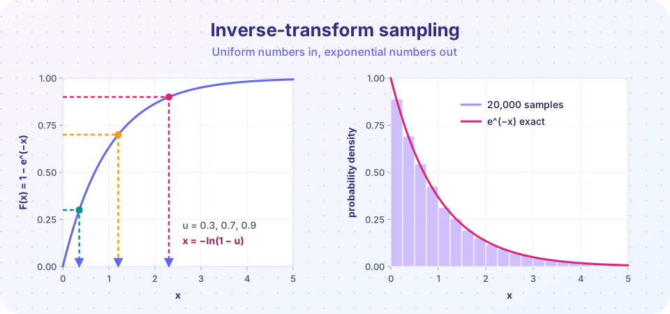
Given a target with CDF F(x), draw u uniformly and return x = F⁻¹(u). Why does it work? The probability that x ≤ a equals the probability that u ≤ F(a), which is F(a): exactly the CDF we wanted.
Example: radioactive decay. A nucleus with mean lifetime τ has the lifetime density f(t) = (1/τ) e^(−t/τ) and CDF F(t) = 1 − e^(−t/τ). Solving F(t) = u gives
t = −τ ln(1 − u)
Since 1 − u is also uniform, many programs use t = −τ ln u. The figure above shows the idea for τ = 1: each uniform u on the vertical axis maps through the curve to a lifetime on the horizontal axis.
Press Run (or Ctrl + Enter) to see the result here.
Program input · what you'd type while the program runs
Type the answers before you press Run, one per line. Each time the program reads a line (with input()), it gets the next line from this box.
Gaussian numbers: Box-Muller
The Gaussian CDF has no elementary inverse, so use a different trick. Take two independent uniforms u₁, u₂:
z₁ = √(−2 ln u₁) cos(2π u₂), z₂ = √(−2 ln u₁) sin(2π u₂)
Both z₁ and z₂ are independent standard normal numbers (mean 0, variance 1). The proof works in polar coordinates: the radius squared of a 2D Gaussian follows an exponential law (which you can sample by inverse transform), and the angle is uniform. To get a Gaussian of mean μ and standard deviation σ, use μ + σ z. In practice, call rng.normal(μ, σ, size); it uses a faster algorithm with the same result.
Rejection sampling
When you can evaluate the density f(x) but cannot invert its CDF, use rejection sampling: pick a simple envelope, throw darts, keep those under the curve.
- Pick
Mwithf(x) ≤ Mon the interval[a, b]. - Draw
xuniformly on[a, b]andyuniformly on[0, M]. - Accept
xify ≤ f(x), otherwise discard it.
The accepted x follow f. The efficiency is the area under f divided by the area of the rectangle, so a tight envelope wastes fewer samples.
Press Run (or Ctrl + Enter) to see the result here.
Program input · what you'd type while the program runs
Type the answers before you press Run, one per line. Each time the program reads a line (with input()), it gets the next line from this box.
Random directions on a sphere
A neutron scatters in a random direction. A tempting recipe, "pick the polar angle θ uniformly in [0, π] and the azimuth φ uniformly in [0, 2π]", is wrong: it piles points near the poles, because the ring at polar angle θ has circumference 2π sin θ. The correct recipe draws cos θ uniformly in [−1, 1] (this is Archimedes' hat-box theorem: equal heights cut equal areas on a sphere).
Press Run (or Ctrl + Enter) to see the result here.
Program input · what you'd type while the program runs
Type the answers before you press Run, one per line. Each time the program reads a line (with input()), it gets the next line from this box.
Common misconceptions
"If the numbers look random, any transformation of them is fine." The θ-uniform sphere example shows that a plausible recipe can be biased. Verify distributions with a histogram and known moments.
"Seed with the clock to be safe." For research, record the seed so the result can be reproduced.
"rng.random() can return 1.0." It returns values in [0, 1): never exactly 1. That matters for log(1 − u) (safe) versus log(u) (could be log(0), though the chance is negligible).
Check your understanding
Quick check · 5 questions
of 5 answered You scored / 5 · perfect!
-
1. What does the inverse-transform method compute?
Solve F(x) = u for x. The resulting x has CDF F. -
2. For exponential lifetimes with mean tau, a sample is
Inverting F(t) = 1 - exp(-t/tau) gives t = -tau ln(1 - u). -
3. Why is picking theta uniformly in [0, pi] wrong for directions on a sphere?
A ring at polar angle theta has circumference 2 pi sin(theta). Draw cos(theta) uniformly instead. -
4. In rejection sampling, what does the acceptance rate depend on?
A tight envelope rejects fewer points. -
5. How should you generate independent random streams for parallel workers?
spawn produces statistically independent child streams.
Summary
- PRNGs are deterministic; seed them for reproducibility and use
np.random.default_rng. - Inverse transform:
x = F⁻¹(u); for decay,t = −τ ln(1 − u). - Box-Muller turns two uniforms into two Gaussians; rejection sampling needs only the density.
- Uniform directions need
cos θuniform, notθ. - Always check a sampler with a histogram and known moments.
Next: Monte Carlo Integration
Track your progress
Create a free account to tick off lessons and pick up where you left off on any device.
of Computational Physics lessons completed