


















Lesson 4 of 47 · Getting Started
Plotting Physics Data with Matplotlib
Learn to draw clear physics plots with Matplotlib: labeled axes with units, error bars, log scales, subplots and residuals, with runnable examples and a checklist.
A number in a table is hard to judge. The same number in a plot shows its trend, its noise and its outliers at a glance. In computational physics you will plot constantly: to see whether a trajectory looks sensible, whether an error shrinks as it should, whether a fit follows the data.
This lesson covers the plotting habits that turn a quick sketch into a figure a colleague can read without asking you what it means.
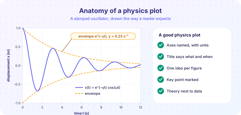
What you will learn
- Build a figure with
plt.plot,plt.scatterandplt.errorbar. - Label axes with quantity and unit, and add legends and annotations.
- Choose linear, semi-log or log-log axes to match the physics.
- Show a fit together with its residuals.
Key terms
Axes: the rectangle holding the data, with its two coordinate axes.
Error bar: a line showing the uncertainty of a measured point.
Residual: data minus model; a good fit leaves residuals scattered around zero.
Log-log plot: both axes logarithmic; a power law y = a x^p becomes a straight line of slope p.
The minimum a plot needs
Every physics plot should answer four questions without a caption.
- What is plotted? Both axes carry a name and a unit:
time t (s),energy E (J). A dimensionless quantity says so:ratio T/T0. - Which curve is which? Use a legend or direct labels.
- What is the point? A title or an annotation names the key feature.
- Can I trust the scale? Start axes at sensible values, avoid overlapping ticks, and use enough resolution.
Matplotlib's plt.plot(x, y) draws a line through points. Use marker="o" when each point is a real measurement, and a smooth line for a computed curve with many points.
Press Run (or Ctrl + Enter) to see the result here.
Program input · what you'd type while the program runs
Type the answers before you press Run, one per line. Each time the program reads a line (with input()), it gets the next line from this box.
Showing data with uncertainty
Measurements come with uncertainty, and the plot should say so. plt.errorbar(x, y, yerr=sigma, fmt="o") draws points with vertical bars. In the next example the "data" are synthetic: we generate a straight line plus random noise, so we know the true answer. This is a standard way to test analysis code before using it on real measurements.
A least-squares line fit minimizes the sum of squared residuals. np.polyfit(x, y, 1) returns slope and intercept.
Press Run (or Ctrl + Enter) to see the result here.
Program input · what you'd type while the program runs
Type the answers before you press Run, one per line. Each time the program reads a line (with input()), it gets the next line from this box.
If the residuals show a pattern (a curve, a trend) instead of random scatter, the model is missing something. That is the most useful thing a residual plot can tell you.
Choosing axes: linear, semi-log, log-log
The right axes make the physics visible.
| Relation | Looks like | Use |
|---|---|---|
y = a x + b |
straight line | linear axes |
y = A e^(-x/τ) |
straight line, slope -1/τ |
semi-log (plt.semilogy) |
y = a x^p |
straight line, slope p |
log-log (plt.loglog) |
For a pendulum, T = 2π √(L/g), so T ∝ L^(1/2). On a log-log plot of T against L you should see a line with slope 0.5. The slope of a straight line on log-log axes is the exponent.
Press Run (or Ctrl + Enter) to see the result here.
Program input · what you'd type while the program runs
Type the answers before you press Run, one per line. Each time the program reads a line (with input()), it gets the next line from this box.
Common misconceptions
"A plot with a smooth curve proves the model is right." A smooth curve through noisy data can hide a poor fit. Always look at residuals.
"Plot defaults are fine." Without axis labels and units the plot is unreadable to anyone who did not write the code, including you in a month.
"Log axes just make plots look nicer." They change what you can see. A power law and an exponential look alike on linear axes but differ clearly on log-log and semi-log plots.
Check your understanding
Quick check · 4 questions
of 4 answered You scored / 4 · perfect!
-
1. Which axis label follows good practice?
A label should name the quantity and give its unit. -
2. On a log-log plot a power law y = a x^p appears as
Taking logs gives log y = log a + p log x, which is linear with slope p. -
3. What do residuals that curve systematically away from zero tell you?
Random scatter means the fit captures the trend. A pattern means the model has the wrong shape. -
4. Why test analysis code on synthetic data with a known truth?
When the true parameters are known, you can see whether the analysis returns them within the uncertainty.
Summary
- Name every axis with quantity and unit, label curves, and annotate the key point.
- Use
errorbarfor measurements and show residuals under a fit. - Choose log axes when the physics suggests a power law or an exponential.
- Test analysis code on synthetic data first.
Next: Chapter 1 Review
Track your progress
Create a free account to tick off lessons and pick up where you left off on any device.
of Computational Physics lessons completed