


















Lesson 20 of 47 · Monte Carlo Methods
Random Walks and Diffusion
Simulate random walks in one and two dimensions, show that the mean squared distance grows linearly with time, and extract the diffusion coefficient from the simulation.
A grain of pollen in water jitters unpredictably. A drop of ink spreads, a smell crosses a room, heat creeps through a metal rod. Behind all of these is one simple mathematical object: the random walk. Each step is random and independent, yet the collective behavior of many walkers is perfectly regular. This is how Monte Carlo connects microscopic randomness to macroscopic laws.
What you will learn
- How to simulate random walks in 1D and 2D with vectorized NumPy.
- The central results
⟨x⟩ = 0and⟨x²⟩ = N a². - How the walk relates to the diffusion equation and the diffusion coefficient
D. - How to measure
Dfrom a simulation.
Key terms
Random walk: a path made of independent random steps.
Mean squared displacement (MSD): ⟨r²⟩, the average over walkers of the squared distance from the start.
Diffusion coefficient D: a constant (units m²/s) defined by ⟨r²⟩ = 2 d D t in d dimensions.
Brownian motion: the random motion of a small particle in a fluid, driven by molecular collisions.
The one-dimensional walk
A walker starts at x = 0. At each time step it moves +a or −a with equal probability. After N steps its position is a sum x = a (s₁ + s₂ + … + s_N) where each sᵢ = ±1. Because the steps are independent with mean 0 and variance 1:
⟨x⟩ = 0: no drift.⟨x²⟩ = N a²: the variance adds up, so the typical distance grows like√N, notN.
By the central limit theorem, for large N the position is approximately Gaussian with variance N a². The typical spread is a√N. Doubling the typical distance takes four times as many steps.
Press Run (or Ctrl + Enter) to see the result here.
Program input · what you'd type while the program runs
Type the answers before you press Run, one per line. Each time the program reads a line (with input()), it gets the next line from this box.
Two dimensions and the MSD
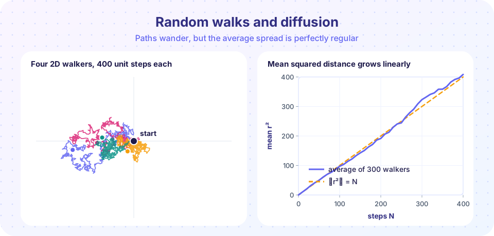
In 2D, let each step have unit length and a uniformly random direction: Δr = (cos φ, sin φ) with φ uniform in [0, 2π). Then ⟨Δx²⟩ + ⟨Δy²⟩ = 1 per step and the squared distance after N steps averages to ⟨r²⟩ = N. Averaging over many walkers gives a clean straight line against N, as the figure shows. The single paths are jagged, but the ensemble average is smooth.
Connecting to diffusion
If each step has length a and takes time τ, then t = N τ and the mean squared displacement is ⟨r²⟩ = N a² = (a²/τ) t. The macroscopic definition of the diffusion coefficient in d dimensions is
⟨r²⟩ = 2 d D t
so for the random walk D = a² / (2 d τ). In d = 2 with a = 1, τ = 1 you expect D = 1/4. The same D appears in the diffusion equation ∂c/∂t = D ∇² c for the concentration c(r, t) of many walkers: you will solve it on a grid in chapter 5. Einstein's 1905 analysis of Brownian motion used exactly this link, and Jean Perrin's measurements of the pollen-like particles' MSD helped establish that atoms are real.
Press Run (or Ctrl + Enter) to see the result here.
Program input · what you'd type while the program runs
Type the answers before you press Run, one per line. Each time the program reads a line (with input()), it gets the next line from this box.
The statistical error is itself a Monte Carlo error that shrinks like 1/√(walkers), so averaging more walkers gives a smoother MSD.
Watch diffusion happen
The interactive demo below releases 400 walkers from the origin. The pink dashed circle has radius √t, the theoretical root-mean-square distance. Notice how the cloud fills the circle and how slowly the radius grows.
Extensions you will meet later
- Biased walks have a drift: a step to the right with probability
p ≠ 1/2gives⟨x⟩ = N a (2p − 1), which models a particle in an electric field. - Absorbing and reflecting boundaries give first-passage times and escape probabilities.
- Recurrence: a simple random walk on a line or a plane returns to the start with probability 1, while in three dimensions it may escape forever (Pólya's theorem).
- Self-avoiding walks model polymer chains: the walk may not revisit a site, and the size grows faster than
√N.
Common misconceptions
"A random walker drifts away linearly with time." The typical distance grows only as √t; the MSD, not the distance, is linear.
"One long walk is as good as many short ones." The MSD is an average over the ensemble, and a single walk has large fluctuations. Average over walkers (or over time windows) before fitting D.
"Diffusion pushes particles." There is no force: the spreading is the statistics of random steps. Concentration gradients appear to drive a flow because more walkers step from the crowded side than from the empty side.
Check your understanding
Quick check · 5 questions
of 5 answered You scored / 5 · perfect!
-
1. After N unit steps of an unbiased 1D random walk, the mean squared displacement is
Variances of independent steps add: each contributes 1, so <x^2> = N. -
2. The typical distance of a random walker from the start grows like
The rms distance is the square root of the MSD, sqrt(N). -
3. In d dimensions the MSD satisfies <r^2> = 2 d D t. For d = 3 and MSD = 6 D t what does the factor 6 represent?
2d = 6 for d = 3. -
4. For a 2D walk with steps of length 1 every time unit, D equals
D = a^2 / (2 d tau) = 1 / (2 * 2) = 1/4. -
5. Why average over many walkers?
The smooth linear law emerges only in the average.
Summary
- An unbiased random walk has
⟨x⟩ = 0and⟨x²⟩ = N a²; the spread grows like√N. - The MSD of an ensemble grows linearly in time:
⟨r²⟩ = 2 d D t. - Measure
Dby fitting the MSD of many walkers; the error shrinks like1/√(walkers). - Random walks are the microscopic picture behind the diffusion equation.
Track your progress
Create a free account to tick off lessons and pick up where you left off on any device.
of Computational Physics lessons completed