


















Lesson 19 of 47 · Monte Carlo Methods
Monte Carlo Integration
Estimate integrals by averaging random samples, report the standard error, see why the 1/sqrt(N) law holds in any dimension, and cut the variance with importance sampling.
Integrals are everywhere in physics: the center of mass of an odd-shaped body, the probability of finding a particle in a region, the partition function of a thermal system. On a grid, the cost of an integral explodes with dimension. Monte Carlo integration trades certainty for scalability: it gives an estimate with a quantifiable statistical error, and that error does not care how many dimensions there are.
What you will learn
- The sample-mean estimator and its standard error.
- Why the error follows
σ/√N, regardless of dimension. - How to estimate a high-dimensional volume.
- How importance sampling reduces the variance.
Key terms
Sample-mean estimator: I ≈ (b − a) · mean(f(xᵢ)) for xᵢ uniform in [a, b].
Standard error: σ_f / √N, estimated from the samples themselves.
Variance reduction: any technique that lowers σ without adding bias.
Importance sampling: draw from a density p(x) that resembles |f| and average f/p.
The sample-mean estimator
For I = ∫ₐᵇ f(x) dx, draw x₁, …, x_N uniformly from [a, b] and compute
I ≈ Î = (b − a) · (1/N) Σ f(xᵢ)
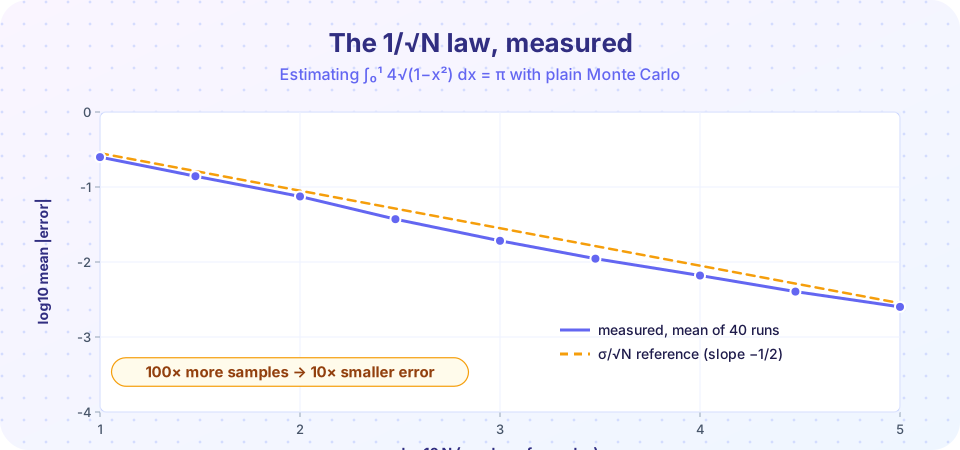
The average (1/N) Σ f(xᵢ) estimates the mean value ⟨f⟩, and the integral is the mean value times the length of the interval. Each f(xᵢ) is a random variable with variance σ², so the estimate has variance σ²/N. In practice you estimate σ from the same samples with np.std(f_vals, ddof=1).
The central limit theorem says Î is approximately normal with that variance, so a good error bar is Î ± σ̂/√N · (b − a), which covers the true value about 68 percent of the time.
Press Run (or Ctrl + Enter) to see the result here.
Program input · what you'd type while the program runs
Type the answers before you press Run, one per line. Each time the program reads a line (with input()), it gets the next line from this box.
The standard error predicts the size of the actual error, though any single run can land farther away: about one run in three has an error above one standard error.
Watching convergence
A good diagnostic is the running mean with its error band. The band narrows like 1/√N, and the estimate should wander inside it.
Press Run (or Ctrl + Enter) to see the result here.
Program input · what you'd type while the program runs
Type the answers before you press Run, one per line. Each time the program reads a line (with input()), it gets the next line from this box.
Why the dimension does not matter
A grid integral with m points per axis in d dimensions uses m^d points, and its error with the trapezoid rule falls like m⁻², which means error ∝ N^(−2/d): terrible for d beyond a few. Monte Carlo's error is σ/√N whatever d is. This is the main reason Monte Carlo is the standard tool for integrals over many particles' coordinates.
A caution: the variance σ² can grow with dimension. To estimate the volume of the unit ball in d dimensions by throwing points in the cube [−1, 1]^d, the fraction that lands inside falls quickly as d grows (the ball fills almost none of the cube), so you need many samples to see any hits.
Press Run (or Ctrl + Enter) to see the result here.
Program input · what you'd type while the program runs
Type the answers before you press Run, one per line. Each time the program reads a line (with input()), it gets the next line from this box.
The estimate keeps working, but the hit fraction drops sharply with d, so the relative error grows. Smarter sampling (importance sampling) is needed in many dimensions.
Importance sampling
Plain sampling wastes effort where f is small. Instead draw from a density p(x) that is large where |f| is large, and average the ratio f/p:
I = ∫ f(x) dx = ∫ (f(x)/p(x)) p(x) dx ≈ (1/N) Σ f(xᵢ)/p(xᵢ), xᵢ ~ p
The estimator is unbiased for any p > 0 where f ≠ 0. Its variance is smallest when p ∝ |f|. Example: I = ∫₀¹ e^(−10x) dx ≈ 0.1. The integrand is large only near x = 0, so plain uniform sampling spends most points where f is nearly zero. Draw instead from the truncated exponential p(x) = a e^(−a x) / (1 − e^(−a)) on [0, 1] with a = 5, which also favors small x, using inverse transform, and average f/p.
Press Run (or Ctrl + Enter) to see the result here.
Program input · what you'd type while the program runs
Type the answers before you press Run, one per line. Each time the program reads a line (with input()), it gets the next line from this box.
For the same N, the importance-sampled estimate has a much smaller standard error: the variance ratio printed above is the factor by which plain sampling would need more samples to match it. A well chosen p is worth far more than a faster computer, while a badly chosen one can make things worse.
Common misconceptions
"Monte Carlo is just an inferior grid method." In a few dimensions, a grid or quad is better. Monte Carlo wins when the dimension is high or the domain is complicated.
"The error bar guarantees the answer." A one-sigma bar contains the truth about 68 percent of the time. Report it as an uncertainty, not a bound.
"Importance sampling is always a win." A poor p that is small where |f| is large can make the variance infinite. Check that f/p is bounded or at least well behaved.
Check your understanding
Quick check · 5 questions
of 5 answered You scored / 5 · perfect!
-
1. A Monte Carlo estimate has standard error 0.02 at N = 10,000. About what is the standard error at N = 1,000,000?
100 times more samples gives 10 times smaller error. -
2. What is the standard error of the sample mean?
Variance of the mean is sigma^2 / N. -
3. Why does the 1/sqrt(N) error law make Monte Carlo useful in high dimensions?
Grid error scales like N^(-2/d) or worse, but Monte Carlo keeps N^(-1/2). -
4. In importance sampling, what do you average?
The ratio f/p corrects for the nonuniform sampling. -
5. Which p(x) minimizes the variance of the importance estimator?
If p is proportional to |f| the ratio f/p is constant, giving zero variance in the ideal case.
Summary
Î = (b − a)·mean(f(xᵢ))with standard errorσ̂/√N.- The
1/√Nlaw holds in any dimension, which is why Monte Carlo is the integration method for many-body problems. - High dimensions raise the variance; use better sampling.
- Importance sampling draws from
p ≈ |f|and averagesf/p. - Report estimate
±error and the seed.
Track your progress
Create a free account to tick off lessons and pick up where you left off on any device.
of Computational Physics lessons completed