


















Lesson 42 of 47 · Projects and Practice
Project: the chaotic double pendulum
Simulate a double pendulum with a fourth-order Runge-Kutta integrator, verify energy conservation, and measure how tiny differences in the start grow exponentially.
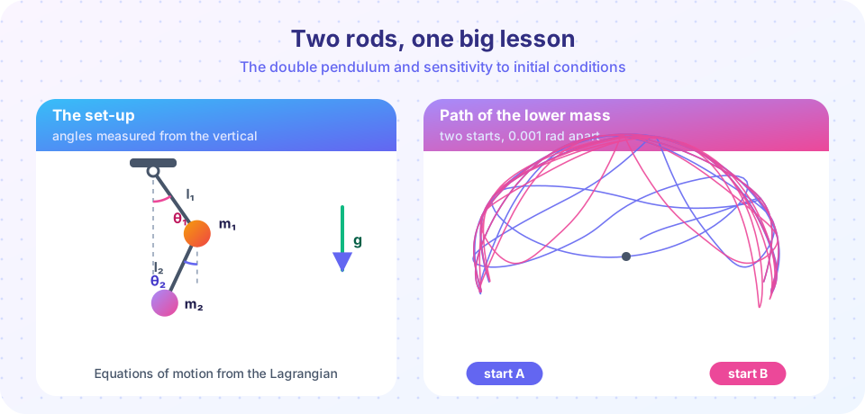
Hang a second pendulum from the end of the first and the simplest toy in physics becomes a source of chaos. Two rods, two masses, no friction: the equations are deterministic, yet two starts that differ by a millionth of a radian soon swing in completely different ways. In this project you will build the simulation, prove it conserves energy, and measure the speed at which nearby trajectories separate. It uses ideas from earlier chapters: integrators (chapter 3), conservation checks (chapter 6) and fitting a slope (chapter 8).
What you will build
- A function that returns the accelerations of both angles.
- A fourth-order Runge-Kutta (RK4) time stepper.
- An energy monitor that tests the code.
- A divergence measurement that estimates how fast chaos grows.
Key terms
Generalized coordinates: the angles θ₁, θ₂ that describe the configuration; the Lagrangian method turns them into equations of motion.
RK4: a fourth-order method that combines four slope estimates per step; the error per unit time scales like Δt⁴.
Chaos: deterministic motion where nearby starts separate exponentially.
Lyapunov exponent λ: the average rate of that separation, δ(t) ≈ δ₀ e^{λt}.
Phase space: the space of all positions and velocities (θ₁, θ₂, ω₁, ω₂).
The equations
Take masses m₁, m₂, rod lengths l₁, l₂ and gravity g. With angles measured from the downward vertical, the Lagrangian method gives
Δ = θ₁ − θ₂,   D = 2m₁ + m₂ − m₂ cos 2Δ

θ₁'' = [ −g(2m₁+m₂) sin θ₁ − m₂ g sin(θ₁ − 2θ₂) − 2 sin Δ · m₂ (ω₂² l₂ + ω₁² l₁ cos Δ) ] / (l₁ D)
θ₂'' = [ 2 sin Δ ( ω₁² l₁ (m₁+m₂) + g (m₁+m₂) cos θ₁ + ω₂² l₂ m₂ cos Δ ) ] / (l₂ D)
The total energy is E = ½(m₁+m₂) l₁² ω₁² + ½ m₂ l₂² ω₂² + m₂ l₁ l₂ ω₁ ω₂ cos Δ − (m₁+m₂) g l₁ cos θ₁ − m₂ g l₂ cos θ₂. It is exactly conserved by the true motion, which makes it the perfect test of your integrator.
RK4 in one paragraph
To advance the state y = (θ₁, θ₂, ω₁, ω₂) with y' = f(y): compute k₁ = f(y), k₂ = f(y + ½Δt k₁), k₃ = f(y + ½Δt k₂), k₄ = f(y + Δt k₃), then y ← y + (Δt/6)(k₁ + 2k₂ + 2k₃ + k₄). Four force evaluations per step, but the error falls as Δt⁴: halving the step makes the error about 16 times smaller. RK4 is not symplectic, so over very long runs the energy slowly drifts; for a short chaotic run it is an excellent choice.
Measuring chaos
Start two pendulums, A and B, with θ₁ differing by δ₀ = 10⁻⁶. Let δ(t) be the distance between their states in phase space. If the motion is chaotic, ln δ(t) rises roughly linearly, and the slope is the largest Lyapunov exponent. Two cautions: once δ reaches the size of the whole attractor (order 1) it cannot grow further, so fit only the middle section; and RK4 round-off also grows exponentially, so the answer for very long times is not trustworthy. This limits how far ahead anyone can predict a chaotic system, and it is why weather forecasts degrade after about two weeks.
Common misconceptions
- "Chaotic means random." The equations are fully deterministic; the unpredictability comes from sensitivity to the start.
- "A tiny energy error means the trajectory is right." Energy can be conserved while the individual path is wrong after a few Lyapunov times.
- "Every double pendulum is chaotic." At small angles the motion is nearly regular (two normal modes); chaos needs enough energy.
- "Use a smaller step and the paths will agree forever." They agree longer, but not forever: the limit grows only logarithmically with accuracy.
Try it
The solver and the energy test. We integrate for 20 seconds from a high-energy start with two time steps. If your implementation is right, the energy drift should be tiny and should fall steeply (a factor of 16 or more) each time the step is halved.
Press Run (or Ctrl + Enter) to see the result here.
Program input · what you'd type while the program runs
Type the answers before you press Run, one per line. Each time the program reads a line (with input()), it gets the next line from this box.
Now the chaos measurement. Two pendulums differ by 10⁻⁶ rad in θ₁. We follow ln δ(t) and fit its slope on the growth phase, for a high-energy start and for a low-energy start where the motion is regular.
Press Run (or Ctrl + Enter) to see the result here.
Program input · what you'd type while the program runs
Type the answers before you press Run, one per line. Each time the program reads a line (with input()), it gets the next line from this box.
Finally a cross-check against an independent adaptive solver. If both agree for the first few seconds, the implementation is trustworthy; where they part, you are looking at chaos amplifying round-off.
Press Run (or Ctrl + Enter) to see the result here.
Program input · what you'd type while the program runs
Type the answers before you press Run, one per line. Each time the program reads a line (with input()), it gets the next line from this box.
Check your understanding
Quick check · 5 questions
of 5 answered You scored / 5 · perfect!
-
1. RK4 is a fourth-order method. If you halve Δt, the error per unit time falls by about...
Error ∝ Δt⁴, so halving Δt divides it by 2⁴ = 16. -
2. What is the Lyapunov exponent?
δ(t) ≈ δ₀ e^{λt}; λ > 0 signals chaos. -
3. Why is energy conservation a good test of the code?
A conservative system with no friction has constant E; changes expose mistakes. -
4. Two chaotic runs differing by 1e-6 separate to order 1 after about 10 s. With initial difference 1e-12, the time roughly...
ln(10⁶) more e-folds are needed, so the prediction horizon grows only logarithmically (about twice as long). -
5. At very small angles the double pendulum motion is...
At small amplitudes the system behaves like two coupled linear oscillators.
Summary
- Build the double pendulum from the Lagrangian equations and advance it with RK4.
- Test the code with energy conservation and an independent solver.
- Chaos is exponential separation of nearby starts; fit the slope of
ln δ(t)in the growth phase to get λ. - Prediction horizons grow only logarithmically with initial accuracy.
Track your progress
Create a free account to tick off lessons and pick up where you left off on any device.
of Computational Physics lessons completed