


















Lesson 26 of 47 · Partial Differential Equations
The Laplace equation and relaxation methods
Solve the 2D Laplace equation by relaxation: Jacobi, Gauss-Seidel and successive over-relaxation, with iteration counts and a check against exact symmetry.
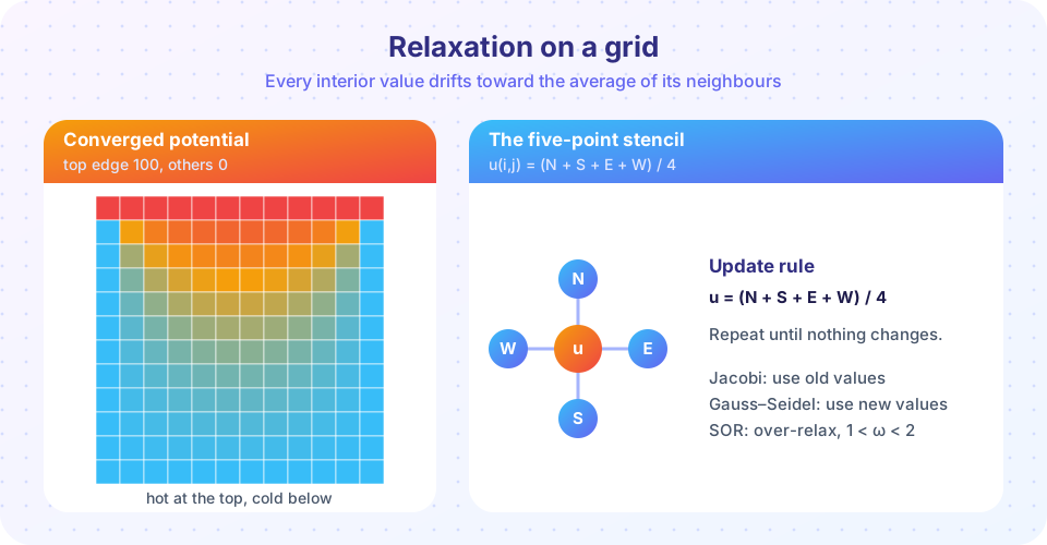
Clamp one edge of a metal plate at 100 degrees and the others at 0, then wait. The temperature settles into a smooth landscape that no longer changes. The same equation describes the electric potential in empty space between charged conductors, the velocity potential of an ideal fluid and a stretched soap film. It is called the Laplace equation, and it has no time in it at all.
Because nothing marches forward, we cannot use a time-stepping scheme. Instead we start with a guess and keep improving it until it stops changing. This is called relaxation.
What you will learn
- What the Laplace equation says and why its solution is the "average of neighbours".
- How Jacobi, Gauss-Seidel and SOR differ and how much faster each is.
- How to choose the over-relaxation factor
ω. - How to check a solution with a symmetry argument.
Key terms
Laplacian: the operator ∇²u = ∂²u/∂x² + ∂²u/∂y².
Harmonic function: a function that satisfies ∇²u = 0. It has no local maxima or minima inside the region.
Relaxation: repeatedly updating values until they stop changing.
Convergence tolerance: the size of the largest change that we accept as "stopped".
Red-black ordering: updating alternate grid points in two sweeps so that each sweep can be vectorized.
From the equation to an average
Write the three-point second difference in x and in y on a grid with equal spacing:
(u[i,j+1] − 2u[i,j] + u[i,j−1]) / h² + (u[i+1,j] − 2u[i,j] + u[i−1,j]) / h² = 0
Rearranged: u[i,j] = ¼ (u[i+1,j] + u[i−1,j] + u[i,j+1] + u[i,j−1]). The value at each interior point is the average of its four neighbours. That is a nice property: a harmonic function never has a bump or dip in the middle, so the extreme values always occur on the boundary (the maximum principle).
Three ways to relax
Jacobi. Compute every new value from the old grid, then replace the old grid all at once. Simple and easy to vectorize, but slow.
Gauss-Seidel. Use new values as soon as they exist. This roughly doubles the speed of convergence.
Successive over-relaxation (SOR). After computing the Gauss-Seidel value g, move further in that direction: u_new = u_old + ω (g − u_old) with 1 < ω < 2. For a square grid of N × N points the best choice is approximately
ω_opt = 2 / (1 + sin(π / (N − 1)))
which is close to 2 for large grids. With the optimal ω, the number of iterations grows like N instead of N², a huge saving. SOR was a breakthrough for early computers solving potential problems in the 1950s.
Common misconceptions
- "Relaxation approaches the solution in time, like heat." The iteration count is not physical time; it is a computational device.
- "More over-relaxation is always faster." With
ω ≥ 2the iteration diverges, and a value just slightly above the optimum slows things down noticeably. - "Tiny change between iterations means the answer is accurate." It means the iteration has slowed down. The true error can still be bigger than your tolerance, especially for Jacobi on large grids.
Try it
We solve the unit square with the top edge at 1 and the other three at 0 using all three methods and count the iterations until the largest change is below 1e-5. The vectorized red-black scheme handles Gauss-Seidel (ω = 1) and SOR.
Press Run (or Ctrl + Enter) to see the result here.
Program input · what you'd type while the program runs
Type the answers before you press Run, one per line. Each time the program reads a line (with input()), it gets the next line from this box.
Now a picture of the converged potential with contour lines (equipotentials), and a symmetry check. If you add the four solutions where one edge is 1 and the other three are 0, you get the solution with all edges at 1, which is the constant 1. By symmetry the four centre values are equal, so each must be 0.25.
Press Run (or Ctrl + Enter) to see the result here.
Program input · what you'd type while the program runs
Type the answers before you press Run, one per line. Each time the program reads a line (with input()), it gets the next line from this box.
Check your understanding
Quick check · 5 questions
of 5 answered You scored / 5 · perfect!
-
1. At the solution of the discrete Laplace equation, each interior value equals...
The five-point stencil rearranges to u = (N + S + E + W) / 4. -
2. What is the difference between Jacobi and Gauss-Seidel?
Gauss-Seidel overwrites values as it sweeps; Jacobi keeps the old grid until the sweep is done. -
3. Which value of the over-relaxation factor ω makes SOR diverge?
SOR converges only for 0 < ω < 2; values at or above 2 diverge. -
4. A square plate has one edge at 100 degrees and the other three at 0. What is the temperature at the centre in the steady state?
Superposing the four rotated problems gives a plate with all edges at 100. By symmetry the four centre values are equal and sum to 100, so each is 25. -
5. The maximum principle says a harmonic function...
Each interior value is an average of neighbours, so it cannot exceed all of them.
Summary
- The Laplace equation
∇²u = 0has no time; its discrete version says each interior value is the average of its four neighbours. - Solve it by relaxation: Jacobi (slow), Gauss-Seidel (about twice as fast) and SOR (far faster with
ω ≈ 2/(1 + sin(π/(N−1)))). - Harmonic functions obey the maximum principle, and symmetry arguments give quick exact checks.
Next: Chapter 5 review
Track your progress
Create a free account to tick off lessons and pick up where you left off on any device.
of Computational Physics lessons completed