


















Lesson 42 of 46 · Projects and Practice
Project: A Link Budget Calculator
Build a tested link budget function for radio links, apply it to Wi-Fi and a geostationary satellite downlink, and explore designs with an interactive calculator.
A link budget is just arithmetic, but arithmetic done carelessly is where real projects go wrong: a wrong unit, a gain subtracted instead of added, a forgotten feeder loss. Turning the budget into a small, tested program removes most of those mistakes and lets you ask "what if" questions in seconds.
In this project you will write a link budget function, test it against hand calculations, apply it to two very different systems (a Wi-Fi link through a wall and a geostationary satellite downlink), and then play with an interactive version.
What you will learn
- Structure a calculation so each term is visible and testable.
- Verify a function with known values before trusting it.
- Handle noise by noise figure or by system temperature.
- Compare systems that differ by 100 dB in path loss.
Key terms
- EIRP: transmit power plus antenna gain, minus feeder loss.
- G/T: receive antenna gain minus 10·log10 of the system noise temperature; the figure of merit of satellite earth stations.
- System noise temperature:
T_sys = T_antenna + T_receiver; noise power isk·T_sys·B. - Unit test: a small check with a known answer.
- Margin: SNR above what the modem needs.
Design the function
Write down the inputs and the equations before the code.
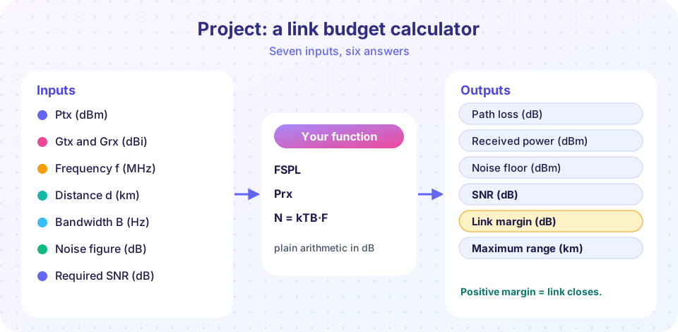
Inputs: transmit power (dBm), transmit and receive antenna gains (dBi), frequency (MHz), distance (km), bandwidth (Hz), noise figure (dB) or system temperature (K), extra losses (dB) such as walls, rain or cables, and required SNR (dB).
Equations:
FSPL = 20·log10(d) + 20·log10(f) + 32.44Prx = Ptx + Gtx + Grx − FSPL − extraN = −174 + 10·log10(B) + NF(dBm) orN = 10·log10(k·T·B / 1 mW)SNR = Prx − N,margin = SNR − requiredLmax = Ptx + Gtx + Grx − extra − (N + required), thend_max = 10^((Lmax − 32.44 − 20·log10(f)) / 20)km
Tests. FSPL at 1 km and 1 GHz must be 92.44 dB; doubling the distance must add 6.02 dB; the noise floor of 1 MHz at NF 0 must be −174 + 60 = −114 dBm. If those pass, you trust the rest.
Apply it
Two scenarios with illustrative numbers (they are plausible, not data from a specific product):
- Wi-Fi in a house: 20 dBm transmitter, 3 dBi antennas, 2.437 GHz, 50 m, an interior wall costing 10 dB, 20 MHz bandwidth, NF 6 dB, 10 dB SNR needed.
- Geostationary TV downlink: 50 dBm (100 W) with a 32 dBi satellite antenna, 12 GHz, 35,786 km, 2 dB atmospheric loss, a 35 dBi home dish, a 36 MHz channel, a system noise temperature of 120 K, 7 dB SNR needed.
The satellite's path loss is about 205 dB against 74 dB for the Wi-Fi link, a 131 dB difference, a factor of more than 10¹³. It works only because every other term is large: a high-power transmitter, a directional antenna at each end and a low-noise receiver.
Common misconceptions
- "The bigger the transmit power, the better the design." Antenna gain and receiver noise are often cheaper and more effective than power.
- "Noise figure and system temperature are different physics." They are two ways to express the same added noise:
T = 290·(10^(NF/10) − 1). - "The budget gives an exact answer." Inputs have tolerances; margins cover them.
- "If the margin is positive, the link always works." Fading and interference move the instantaneous SNR; margins are statistical.
Try it
First, the function with tests, the two scenarios and a bar chart of SNR against the required SNR.
Press Run (or Ctrl + Enter) to see the result here.
Program input · what you'd type while the program runs
Type the answers before you press Run, one per line. Each time the program reads a line (with input()), it gets the next line from this box.
Second, an interactive version. Move the sliders and read the margin; it turns green when the link closes. This is a calculator for the same equations, with noise from the noise figure.
Ideas to extend it
- Add a rain-attenuation term that grows with distance and frequency.
- Add a log-distance model with exponent
ninstead of free space. - Add diversity: two receive antennas reduce the fade margin by a few dB.
- Port the function to JavaScript and build a small web page around it.
- Add a fiber mode with
α·L + connectors + splices.
Check your understanding
Quick check · 4 questions
of 4 answered You scored / 4 · perfect!
-
1. Which test best verifies a free-space path loss function?
Known reference values and scaling properties catch unit and sign mistakes. -
2. A receiver has a system noise temperature of 290 K and a 1 MHz bandwidth. What is its noise power?
k·T·B = 1.38×10⁻²³ × 290 × 10⁶ = 4×10⁻¹⁵ W = −114 dBm. -
3. Why can the satellite link close despite about 205 dB of path loss?
The budget is a sum: large gains and low noise offset the huge loss. -
4. A link has margin −3 dB. Which change would close it most cheaply in free space?
Each +3 dB of power or gain adds 3 dB of margin; the other changes make it worse.
Summary
- Express a link budget as a function and test it against known values before using it.
- Noise can come from a noise figure or from a system temperature; the two are equivalent.
- Systems with very different path loss differ mainly in how many decibels of gain and noise performance they bring.
- An interactive calculator makes trade-offs between power, gain, distance and noise easy to see.
Next: Practice problems
Track your progress
Create a free account to tick off lessons and pick up where you left off on any device.
of Communication Systems lessons completed