


















Lesson 20 of 46 · Sampling and Digital Transmission
Chapter 4 review: Sampling and digital transmission
Review the sampling theorem, aliasing, quantization noise, PCM bit rates, line codes and Nyquist pulses with a recap table and a ten-question quiz.
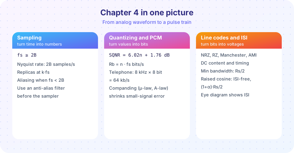
Chapter 4 closed the loop from an analog waveform to a train of voltage pulses ready for a carrier. Three numbers from this chapter come back constantly: the sampling rate (at least 2B), the number of bits (6 dB per bit) and the symbol rate with its bandwidth ((1 + α) Rs / 2). This page gathers them, then checks that you can use them.
What you will learn
- How the chapter's results chain together in one bit-rate and bandwidth calculation.
- Which rules of thumb to know by heart.
- Whether you can apply them to mixed problems.
Recap table
| Step | Rule | Lesson |
|---|---|---|
| Sampling | fs > 2B; alias at distance to nearest multiple of fs |
Sampling theorem |
| Quantization | Δ = 2Vmax/2ⁿ, noise Δ²/12 |
Quantization and PCM |
| SQNR | 6.02 n + 1.76 dB (full-scale sine) |
Quantization and PCM |
| Bit rate | Rb = n · fs |
Quantization and PCM |
| Companding | μ-law (255) and A-law (87.6) | Quantization and PCM |
| Line codes | NRZ, RZ, Manchester, AMI | Line codes |
| Pulse shaping | B = (1 + α) Rs / 2 |
Line codes |
Worked chain. Music of bandwidth 20 kHz: fs = 44.1 kHz; 16 bits, 2 channels gives Rb = 44.1 × 16 × 2 = 1.4112 Mb/s; with binary polar signaling and α = 0.25, B = 1.25 × 1.4112 / 2 ≈ 0.88 MHz.
Try it
The first example runs the chain above for any inputs: sampling rate, bits, channels, levels per symbol and roll-off. Change them to see how each choice moves the bandwidth.
Press Run (or Ctrl + Enter) to see the result here.
Program input · what you'd type while the program runs
Type the answers before you press Run, one per line. Each time the program reads a line (with input()), it gets the next line from this box.
The second example is a mixed drill with answers computed by code, so you can check your hand calculations.
Press Run (or Ctrl + Enter) to see the console output here.
No output.
Check your understanding
Quick check · 10 questions
of 10 answered You scored / 10 · perfect!
-
1. A signal limited to 6 kHz is to be sampled. A valid sampling rate is
fs must be greater than 2B = 12 kHz; 14 kHz qualifies, 12 kHz exactly is the boundary and is not safe. -
2. A 15 kHz tone is sampled at 20 kHz. It appears at
|15 − 20| = 5 kHz. -
3. A 6-bit quantizer and a 7-bit quantizer differ in SQNR by about
Each added bit gives 6.02 dB. -
4. A 16-bit quantizer has Vmax = 1 V. The step size is about
Δ = 2 / 65,536 ≈ 30.5 µV. -
5. Which is true of Manchester coding relative to polar NRZ?
The mid-bit transition doubles the spectral width and gives timing information. -
6. A raised-cosine pulse with α = 0.5 at 2 Msym/s needs
B = (1 + 0.5) × 2 / 2 = 1.5 MHz. -
7. A voice signal is 64 kb/s PCM. Using 4-level signaling the symbol rate is
Four levels carry 2 bits per symbol: 64 / 2 = 32 ksym/s. -
8. Why does μ-law companding help speech?
The compressor stretches small amplitudes so that the uniform quantizer resolves them better. -
9. What does the eye diagram's opening show?
A wide open eye means a decision at the sampling instant is safe. -
10. Which block of the chain loses information irreversibly?
Quantization rounds values; an adequate sampler and a line encoder are reversible.
Summary
- Sample above
2Bafter an anti-aliasing filter; aliases cannot be removed later. - Quantization adds
Δ²/12noise; SQNR improves 6.02 dB per bit. - PCM bit rate
Rb = n fs; line codes and pulse shape set the bandwidth(1 + α) Rs/2. - The remaining chapters of the course (digital modulation, noise and error performance, coding, wireless and optical systems, projects) continue from the course page.
Track your progress
Create a free account to tick off lessons and pick up where you left off on any device.
of Communication Systems lessons completed