


















Lesson 22 of 49 · Network Optimization
Transportation and Assignment Problems
Ship goods from factories to stores at least cost and match workers to jobs: model the transportation and assignment problems as network LPs and solve them in Python.
Two network models appear in almost every supply-chain and staffing course. In the transportation problem several suppliers must ship goods to several customers at the lowest total shipping cost. In the assignment problem each worker must be matched to exactly one job, again at minimum total cost. They are close relatives: assignment is simply a transportation problem in which every supply and demand is 1.
Both problems are linear programs with a special structure, so the optimal solution is automatically made of whole numbers, and fast specialized algorithms exist. In this lesson you formulate each model, solve it with Python, and learn to check the answers.
What you will learn
- How to formulate and solve a transportation problem.
- How to handle unbalanced supply and demand.
- How to formulate and solve an assignment problem.
- Why the LP solutions come out as whole numbers.
Key terms
Supply: the amount a source can send. Demand: the amount a destination must receive.
Balanced problem: total supply equals total demand.
Dummy node: an artificial source or destination added to balance a problem.
Assignment problem: a transportation problem with all supplies and demands equal to 1.
Hungarian algorithm: a classical method for the assignment problem, developed by Kuhn in 1955 from work of the Hungarian mathematicians Kőnig and Egerváry.
The transportation problem
Sunrise Foods has three factories and four stores (example numbers). Factory supplies per week are 40, 30 and 50 units. Store demands are 25, 35, 30 and 30 units. Total supply (120) equals total demand (120), so the problem is balanced. Shipping costs per unit, in dollars, are:
| Store 1 | Store 2 | Store 3 | Store 4 | Supply | |
|---|---|---|---|---|---|
| Factory 1 | 4 | 6 | 9 | 5 | 40 |
| Factory 2 | 7 | 3 | 5 | 8 | 30 |
| Factory 3 | 6 | 8 | 4 | 3 | 50 |
| Demand | 25 | 35 | 30 | 30 |
Variables. x_ij = units shipped from factory i to store j (12 variables).
Objective. Minimize the total shipping cost Σ c_ij · x_ij.
Constraints. Each factory ships exactly its supply (3 equations) and each store receives exactly its demand (4 equations):
Σ_j x_ij = supply_i      for each factory i
Σ_i x_ij = demand_j      for each store j
x_ij ≥ 0
One of the seven equations is redundant (they sum consistently), which is why a transportation solution uses at most 3 + 4 − 1 = 6 routes.
Press Run (or Ctrl + Enter) to see the result here.
Program input · what you'd type while the program runs
Type the answers before you press Run, one per line. Each time the program reads a line (with input()), it gets the next line from this box.
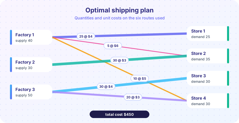
The optimal plan costs $450. For example, Factory 2 ships all its 30 units to Store 2 (cost 3 per unit, the cheapest route in the table), and Factory 3 serves Store 3 and part of Store 4. Check the total by hand: 25·4 + 5·6 + 10·5 + 30·3 + 30·4 + 20·3 = 100 + 30 + 50 + 90 + 120 + 60 = 450. Notice that all shipped quantities are whole numbers, even though the LP never asked for it.
Unbalanced problems
If supply exceeds demand, some supply stays unused: use ≤ for supply rows (or add a dummy store that absorbs the surplus at zero cost). If demand exceeds supply, some demand cannot be met: add a dummy factory that supplies the shortage, usually at a high penalty cost representing lost sales. After balancing, the same model applies.
The heat map below shows the same plan: darker cells are dearer routes, and the pink outlines mark the routes that carry goods.
Press Run (or Ctrl + Enter) to see the result here.
Program input · what you'd type while the program runs
Type the answers before you press Run, one per line. Each time the program reads a line (with input()), it gets the next line from this box.
Reading the plan
Cells with positive shipments are the basic cells in the simplex language. Specialized methods such as the stepping-stone and MODI methods work directly on the table: start with any feasible plan (the northwest-corner or least-cost rule), and test each unused cell to see if shipping one unit there would lower the cost, rerouting along a loop to keep supply and demand balanced. They are the simplex method specialized to a table, and by hand they are practical for small problems.
The assignment problem
Four workers must be given four jobs, one job per worker. Times in hours (example numbers) are:
| Job 1 | Job 2 | Job 3 | Job 4 | |
|---|---|---|---|---|
| Worker A | 9 | 11 | 14 | 11 |
| Worker B | 6 | 15 | 13 | 13 |
| Worker C | 12 | 13 | 6 | 8 |
| Worker D | 11 | 9 | 10 | 12 |
Let x_ij = 1 if worker i does job j, else 0. Minimize Σ c_ij · x_ij subject to each worker doing exactly one job (Σ_j x_ij = 1) and each job being done by exactly one worker (Σ_i x_ij = 1). It looks like an integer program with 16 binary variables, but the LP relaxation always has an optimal solution with 0/1 values, so you can use plain linear programming.
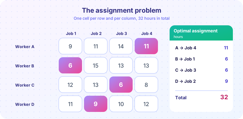
With 4 workers there are 4! = 24 possible assignments, so we can check the answer by brute force. With 20 workers there would be 20! ≈ 2.4 × 10¹⁸, which is why we need the Hungarian algorithm, which solves the problem in time proportional to n³.
Press Run (or Ctrl + Enter) to see the result here.
Program input · what you'd type while the program runs
Type the answers before you press Run, one per line. Each time the program reads a line (with input()), it gets the next line from this box.
The best total is 32 hours: A does Job 4 (11), B does Job 1 (6), C does Job 3 (6) and D does Job 2 (9). Several assignments can tie in other tables; the solver returns one of them.
Why the Hungarian algorithm works (the key idea)
If you subtract the same number from every entry of a row (or column) of the cost table, every complete assignment changes by that same number, so the best assignment is unchanged. The algorithm uses this to create zeros: subtract each row's minimum, then each column's minimum. If you can pick one zero in each row and column, you have an optimal assignment, since no cost can be below zero. If not, the algorithm adjusts the table in a way that creates new zeros while keeping every entry nonnegative, until a full assignment of zeros appears.
Press Run (or Ctrl + Enter) to see the result here.
Program input · what you'd type while the program runs
Type the answers before you press Run, one per line. Each time the program reads a line (with input()), it gets the next line from this box.
The reductions give the lower bound row_min.sum() + col_min.sum(): no assignment can cost less. When the zeros of the reduced table allow a complete selection (one zero per row and per column, as in the matrix of this example), the bound is reached and the assignment is optimal.
Why integer solutions come for free
In both problems each variable x_ij appears in exactly two constraints (its row and its column), each time with coefficient 1. Such a matrix is totally unimodular: every square submatrix has determinant 0, +1 or −1. Combined with integer right-hand sides (supplies, demands, 1s), this guarantees that every corner of the feasible region has integer coordinates, so simplex always lands on an integer solution. The practical message: when you recognize a transportation or assignment structure, use the LP and skip integer programming.
Variations you will meet
- Capacities on routes: add
x_ij ≤ u_ij. - Transshipment: goods can pass through intermediate warehouses; it is a general minimum-cost flow problem.
- Maximization: profit instead of cost; negate and minimize, or switch the objective.
- Unequal sizes: more jobs than workers; add dummy workers with zero cost.
- Side constraints: "worker A cannot do Job 2": set that cost to a very large number, or fix
x_ij = 0.
Common misconceptions
"I must add integer constraints for whole-unit shipments." For the transportation problem with integer supplies and demands, the LP optimum is already integer.
"The cheapest route should be used as much as possible." It will be, up to supply and demand limits, but other routes must fill what remains; greedy shipping is usually not optimal.
"The assignment problem can only be solved by checking all permutations." The Hungarian algorithm needs about n³ operations.
Check your understanding
Quick check · 5 questions
of 5 answered You scored / 5 · perfect!
-
1. In a balanced transportation problem, what must be true?
Balanced means total supply = total demand, so every unit produced is shipped and every demand is met exactly. -
2. How many routes does an optimal basic solution of a 3-by-4 transportation problem use, at most?
At most m + n − 1 = 3 + 4 − 1 = 6 routes are used. -
3. How do you balance a problem where supply exceeds demand?
The dummy destination takes the surplus, making total supply and demand equal. -
4. What is the optimal total time for the example assignment problem?
A-4 (11) + B-1 (6) + C-3 (6) + D-2 (9) = 32. -
5. Why do assignment LPs give 0/1 solutions without integer constraints?
Total unimodularity ensures integer corner points for integer data.
Summary
- The transportation problem ships goods at minimum cost subject to supplies and demands; the example costs $450.
- Unbalanced problems are balanced with dummy sources or destinations.
- The assignment problem matches workers to jobs one-to-one; the example optimum is 32 hours.
- Both are network LPs whose optimal solutions are integers; the Hungarian algorithm solves assignment in
n³steps. - Row and column reductions show a lower bound on the assignment cost.
Next: Chapter 4 Review
Track your progress
Create a free account to tick off lessons and pick up where you left off on any device.
of Operations Research lessons completed