


















Lesson 31 of 49 · Queueing and Simulation
The M/M/1 Queue: One Server, Exact Answers
Learn the M/M/1 queue: derive the steady-state distribution, compute L, Lq, W and Wq, apply Little's law and choose a service rate that balances costs.
The M/M/1 queue is the "hydrogen atom" of queueing theory: the simplest model that is still realistic enough to teach you something true. Customers arrive randomly, one server serves them one at a time, service times are random, and the waiting room is unlimited. Despite the simplicity, its formulas reveal a lesson every manager should know: pushing a server toward full utilization is expensive in waiting time.
This lesson explains the notation, derives the key result in a few lines, and uses it to size a service.
What you will learn
- What the letters in "M/M/1" mean and which assumptions they carry.
- How to compute
ρ,L,Lq,WandWqand how Little's law links them. - How to find the chance of having
ncustomers and the chance of waiting longer thant. - How to balance server cost against waiting cost.
Key terms
Kendall notation: A/S/c, where A describes arrivals, S the service times and c the number of servers. M stands for Markovian (memoryless), meaning exponential times.
Poisson process: random arrivals at constant average rate; the gaps between arrivals are exponentially distributed.
Little's law: L = λ W, the average number in a stable system equals the arrival rate times the average time in the system.
Stability: the queue has a steady state only if ρ = λ/μ < 1.
The model and its notation
In "M/M/1" the first M says that arrivals form a Poisson process with rate λ: gaps between arrivals are exponential with mean 1/λ. The second M says that service times are exponential with mean 1/μ. The 1 means one server. The queue has infinite room and is served first come first served.
The exponential distribution is memoryless: no matter how long a customer has been in service, the expected remaining time is still 1/μ. This is not always realistic (a haircut takes some minimum time), but it makes the mathematics easy, and the answers are a good first approximation.
Where the formulas come from
Let p_n be the long-run fraction of time with n customers in the system. In steady state, the rate at which the system moves from n − 1 to n equals the rate at which it moves back from n to n − 1:
λ · p_{n−1} = μ · p_n so p_n = ρ · p_{n−1} with ρ = λ/μ
Applying this repeatedly gives p_n = ρⁿ p_0. The probabilities must add to 1, and Σ ρⁿ = 1/(1 − ρ) for ρ < 1, so p_0 = 1 − ρ and
p_n = (1 − ρ) ρⁿ
Two facts follow right away: the server is idle a fraction 1 − ρ of the time, and the chance of at least k customers in the system is ρᵏ.
The average number in the system is L = Σ n p_n = ρ / (1 − ρ). The other measures follow from it and from Little's law:
| Measure | Symbol | Formula |
|---|---|---|
| Utilization | ρ |
λ / μ |
| Customers in system | L |
ρ / (1 − ρ) |
| Customers waiting in line | Lq |
ρ² / (1 − ρ) |
| Time in system | W |
1 / (μ − λ) |
| Time waiting in line | Wq |
ρ / (μ − λ) |
The relationships L = λW, Lq = λWq and W = Wq + 1/μ tie the rows together. Little's law is remarkably general: it holds for almost any stable system, whatever the arrival and service distributions are.
A worked example
A walk-in clinic receives λ = 5 patients per hour. The doctor treats μ = 6 per hour.
ρ = 5/6 ≈ 0.833: the doctor is busy 83 percent of the time.L = 0.833 / 0.167 = 5patients in the clinic on average.Lq = 0.833² / 0.167 ≈ 4.17of them waiting.W = 1 / (6 − 5) = 1hour in the clinic.Wq = 0.833 / 1 ≈ 0.833hour, that is 50 minutes in the waiting room, to receive a 10-minute treatment.
Check with Little's law: L = λW = 5 × 1 = 5. ✓. The probability that a patient finds at least 3 others ahead is ρ³ ≈ 0.58.
Try it
Compute the table of formulas and compare it with a simulation of 200,000 patients.
Press Run (or Ctrl + Enter) to see the result here.
Program input · what you'd type while the program runs
Type the answers before you press Run, one per line. Each time the program reads a line (with input()), it gets the next line from this box.
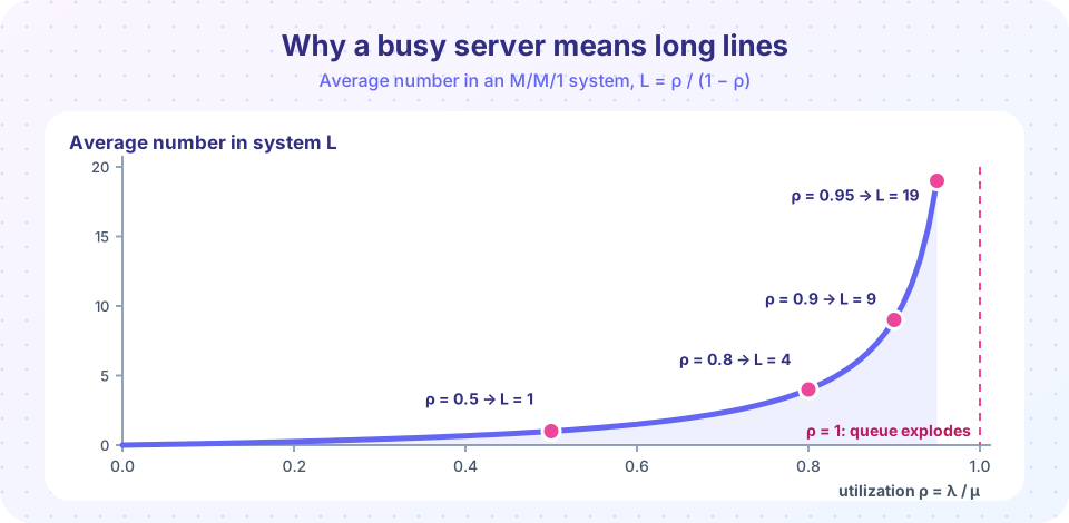
The simulated wait lands close to the formula, and the sweep shows the steep climb from the figure above.
Beyond averages: the distribution of the wait
Averages hide what customers feel. In an M/M/1 queue the time in the system is exponentially distributed with rate μ − λ, so the chance a customer waits more than t in the system is e^{−(μ − λ)t}. For the clinic, P(W > 2 hours) = e^{−2} ≈ 0.135: more than one patient in eight stays over two hours even though the average is one hour. Service-level promises such as "90 percent of customers within 20 minutes" must use the distribution, not the mean.
Balancing costs
How fast should the server be? A faster server costs more, but shortens the line. Suppose waiting costs $20 per customer per hour, arrivals are λ = 4 per hour, and a server working at speed μ costs $6 per unit of μ per hour. The hourly cost is
TC(μ) = 6μ + 20 · L = 6μ + 20 · λ/(μ − λ)
Press Run (or Ctrl + Enter) to see the result here.
Program input · what you'd type while the program runs
Type the answers before you press Run, one per line. Each time the program reads a line (with input()), it gets the next line from this box.
The balance point sits where one extra unit of capacity saves exactly as much waiting cost as it costs. Because the waiting-cost curve is so steep near μ = λ, the best choice leaves a comfortable gap between capacity and demand.
Where M/M/1 stops being true
- Arrivals that are scheduled (appointments) are less bursty than Poisson, so lines are shorter than predicted.
- Service times that are nearly constant cut the average wait roughly in half, compared with exponential times at the same mean (the Pollaczek-Khinchine formula; the simulation lesson shows it).
- Limited waiting rooms, impatient customers and priorities need other models.
The M/M/1 numbers are best used as a quick, slightly pessimistic estimate and a sanity check for bigger models.
A second worked example
An online help chat has one agent who resolves 5 chats an hour (μ = 5), and customers arrive at 4 per hour (λ = 4). Then ρ = 0.8, L = 4, Lq = 3.2, W = 1 hour and Wq = 0.8 hour, which is 48 minutes in the queue for a 12-minute chat. The chance that a customer has to wait at all is ρ = 0.8: four customers in five find the agent busy. The chance that the total time exceeds 2 hours is e^{−(5 − 4) × 2} = e^{−2} ≈ 0.135.
Now suppose the company does nothing but grows: arrivals rise by 10 percent to λ = 4.4. Utilization goes from 0.80 to 0.88, and W = 1/(5 − 4.4) ≈ 1.67 hours. A 10 percent increase in demand raises the average time by about two thirds. This is the lesson of the curve at the top of the page: near full utilization small changes in load have large effects, so a service that "has been fine so far" can collapse after a modest increase in demand.
Reading the formulas
W = 1/(μ − λ)depends only on the gap between capacity and demand. Doubling bothλandμhalvesW, because the same relative gap is measured against twice the speed.Wq = ρ · W: the time in line is the fractionρof the total time, since the rest is the service itself.- The queue is longest when the server is busiest, and the average hides the random swings: in the simulation lesson you will see runs of several customers in a row with long waits.
Common misconceptions
"Utilization of 100 percent is the efficient target." At ρ = 1 the average queue is infinite. Practical targets are often 70 to 85 percent when waiting is costly.
"Wq and W are the same." W includes the service time. W = Wq + 1/μ.
"The average wait is what most customers experience." The distribution has a long tail: a sizable minority wait several times the mean.
Check your understanding
Quick check · 5 questions
of 5 answered You scored / 5 · perfect!
-
1. λ = 3 per hour and μ = 4 per hour. What is L?
ρ = 0.75 and L = ρ/(1 − ρ) = 0.75/0.25 = 3. -
2. For the same queue, what is W?
W = 1/(μ − λ) = 1/(4 − 3) = 1 hour. Check: L = λW = 3 × 1. -
3. An M/M/1 queue has ρ = 0.6. What fraction of the time is the server idle?
p_0 = 1 − ρ = 0.4. -
4. On average 20 customers are in a shop and each stays 10 minutes. What is the arrival rate?
Little's law: λ = L/W = 20/10 = 2 per minute. -
5. What happens to Wq when λ is close to μ?
Wq = ρ/(μ − λ) grows without bound as μ − λ approaches 0.
Summary
- M/M/1 means Poisson arrivals, exponential service, one server; it is stable only if
ρ = λ/μ < 1. p_n = (1 − ρ)ρⁿ,L = ρ/(1 − ρ),W = 1/(μ − λ),Wq = ρ/(μ − λ), and Little's lawL = λWties them together.- Waiting explodes as utilization approaches 1, and the wait distribution has a long tail.
- Server speed should balance capacity cost against waiting cost.
Track your progress
Create a free account to tick off lessons and pick up where you left off on any device.
of Operations Research lessons completed