


















Lesson 48 of 49 · Projects and Practice
Cheat Sheet: Operations Research on One Page
A one-page cheat sheet for operations research chapters 5 to 8: inventory, scheduling, queueing, simulation, decisions, games and heuristics, with a reusable formula toolbox.
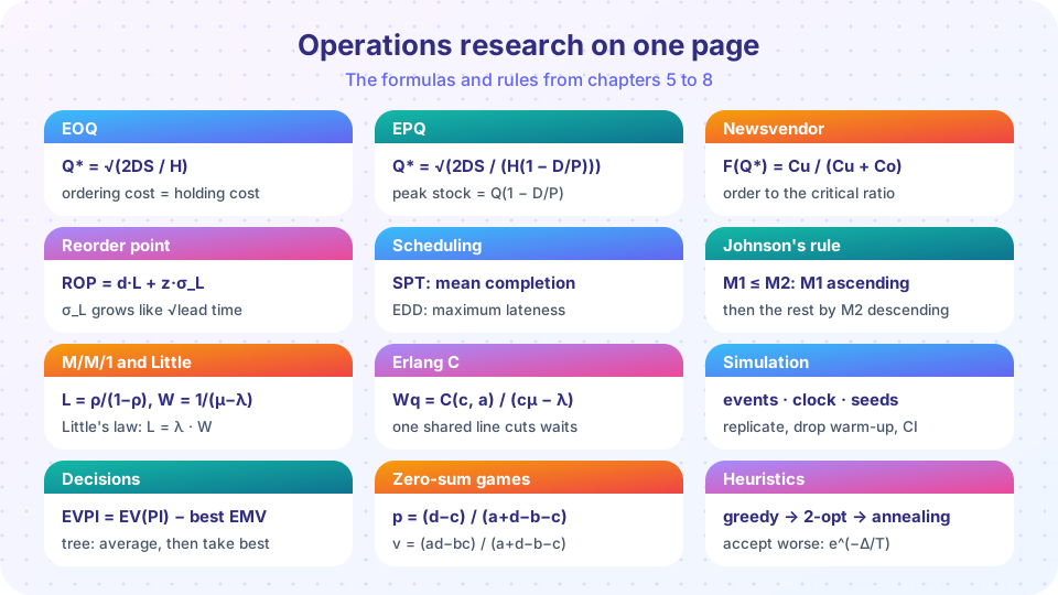
When you are in the middle of a problem, you need the formula and its conditions, not the story behind it. This lesson is a one-page reference for chapters 5 to 8: a poster, a table of "when to use what", a short list of checks that catch most errors and a small Python toolbox that implements every formula. Print the poster, or keep it open beside you while you solve problems.
What you will learn
- To pick the right model for a problem in a few seconds.
- To recall the formulas with their symbols and conditions.
- To run a checklist that catches common mistakes.
Key terms
D, S, H: demand per year, cost per order, holding cost per unit per year.
λ, μ, c, ρ: arrival rate, service rate per server, number of servers, utilization.
Cu, Co: underage and overage cost per unit.
Δ, T: the cost change of a move and the temperature in annealing.
Which model for which problem?
| If the problem says... | Use | Chapter |
|---|---|---|
| Steady demand, fixed cost per order, delivery at once | EOQ | 5 |
| Own factory makes the stock gradually | EPQ | 5 |
| Supplier price drops for larger orders | EOQ with discount procedure | 5 |
| One selling season, random demand | Newsvendor critical ratio | 5 |
| Repeated orders, random demand, delivery delay | Reorder point and safety stock | 5 |
| Order jobs on one machine | SPT (average completion), EDD (lateness) | 5 |
| Two machines in series | Johnson's rule | 5 |
| Random arrivals, one server | M/M/1 formulas | 6 |
| Random arrivals, several servers, one line | Erlang C | 6 |
| Complicated rules, breaks, priorities | Discrete-event simulation | 6 |
| Choose under uncertainty, probabilities known | EMV and a decision tree | 7 |
| Is a forecast worth buying? | EVPI, EVSI | 7 |
| Two opposed players | Saddle point or mixed strategy | 7 |
| NP-hard, large instance, answer needed soon | Greedy, local search, annealing | 8 |
| A messy business question | The five-step OR workflow | 8 |
The formulas, grouped
Inventory (chapter 5)
- EOQ:
Q* = √(2DS/H),TC* = √(2DSH). At the optimum, ordering cost equals holding cost.TC(Q)/TC* = (r + 1/r)/2withr = Q/Q*. - EPQ:
Q* = √(2DS / (H(1 − D/P))), peak stockQ(1 − D/P). - Quantity discounts (all-units): per price level compute the EOQ, clamp it into the allowed range, add
D × price, compare totals. - Newsvendor:
F(Q*) = Cu/(Cu + Co), for normal demandQ* = μ + zσ. - Reorder point:
ROP = d·L + z·σ_L, withσ_L = σ_period · √(number of periods).
Scheduling (chapter 5)
- SPT minimizes mean completion time; EDD minimizes maximum lateness.
- Johnson (two machines): put jobs with
M1 ≤ M2first in ascendingM1, then the rest in descendingM2.
Queues and simulation (chapter 6)
- M/M/1:
ρ = λ/μ,L = ρ/(1 − ρ),Lq = ρ²/(1 − ρ),W = 1/(μ − λ),Wq = ρ/(μ − λ),P(n ≥ k) = ρᵏ. - Little:
L = λW,Lq = λWq. - Erlang C:
a = λ/μ,C(c, a) = [(aᶜ/c!)/(1 − ρ)] / [Σ_{k<c} aᵏ/k! + (aᶜ/c!)/(1 − ρ)],Wq = C/(cμ − λ),P(Wq > t) = C·e^{−(cμ − λ)t}. - Simulation: validate, drop a warm-up, run replications, report
x̄ ± t·s/√n.
Decisions and games (chapter 7)
- EMV:
Σ p_i · payoff_i. EVPI:EV(perfect information) − best EMV. - Criteria: maximin (pessimist), maximax (optimist), Hurwicz
α·best + (1 − α)·worst, Laplace (equal chances), minimax regret. - Zero-sum 2 x 2 (no saddle point):
p = (d − c)/(a + d − b − c),v = (ad − bc)/(a + d − b − c).
Heuristics (chapter 8)
- Gap:
100 × (value − best)/best. - Annealing: accept a worse move with probability
exp(−Δ/T); cool withT ← αT; keep the best solution seen. - Tours:
(n − 1)!/2distinct round trips; nearest neighbor then 2-opt is a good start.
A toolbox you can reuse
The functions below implement the course's formulas. Copy them into your own scripts.
Press Run (or Ctrl + Enter) to see the result here.
Program input · what you'd type while the program runs
Type the answers before you press Run, one per line. Each time the program reads a line (with input()), it gets the next line from this box.
Each printed line reproduces a worked example from the course, so you can see at a glance that the toolbox is right: 774.6 and $1,549 for the EOQ, 217.2 for the newsvendor, 246.5 for the reorder point, 21.07 minutes for the three-agent help line, and so on.
Ten checks that catch most mistakes
- Units: are demand, holding cost and time all per year (or all per day)?
- Stability: is
λ < cμ? If not, the queue formulas do not apply. - Ranges: does an EOQ computed at a discounted price lie in that price's range?
- Zero tests: does the answer behave sensibly if demand is zero or the server is infinitely fast?
- Little check: does
L = λWhold between your two answers? - Square roots: did you take the square root of variance, not add standard deviations?
- Which service level? Cycle service level, fill rate or a call-center target?
- Saddle point first: before computing a mixed strategy, check maximin = minimax.
- Best so far: does the heuristic return the best solution seen, not just the last one?
- Say the assumptions: every number in your report should come with the conditions under which it holds.
A short list of rules of thumb
- Inventory cost is flat near the optimum: a convenient pack size is nearly as good as the exact EOQ.
- Keep utilization below about 85 percent where waiting is costly.
- Pool servers and stocks whenever you can.
- Reduce variability before adding capacity.
- A good answer in time beats a perfect answer too late.
Three quick worked examples
Example 1 (inventory). A bakery uses 7,200 kg of flour a year, an order costs $36 and holding costs $0.50 per kg per year. Q* = √(2 × 7,200 × 36 / 0.5) = √1,036,800 ≈ 1,018 kg, about 7 orders a year, cost √(2 × 7,200 × 36 × 0.5) ≈ $509.
Example 2 (queue). A booth gets 9 customers an hour and serves 12 an hour. ρ = 0.75, L = 3, W = 1/(12 − 9) = 1/3 hour = 20 minutes, and Wq = 0.75/3 = 0.25 hour = 15 minutes. Little's law check: L = λW = 9 × 1/3 = 3. ✓
Example 3 (decision). Option A pays 90 or 10 with equal probability; option B pays 60 for certain. EMV(A) = 50 and EMV(B) = 60, so B is better. With perfect information you would take A when it pays 90 and B otherwise, so the expected payoff is 0.5 × 90 + 0.5 × 60 = 75, and EVPI = 75 − 60 = 15.
How to use the sheet in an exam or a project
Start from the table "which model for which problem", write down the model and its conditions, and only then reach for the formula. When an answer looks odd, run through the ten checks. For a project, put the assumptions of the model on the first page of the report, next to the result, so that a reader can see when the answer applies.
Symbols at a glance
Many errors come from mixing up symbols that look alike. Capital D is demand per year, while lowercase d is demand per day in the reorder-point formula and the entry in the lower right of a game matrix. S is a cost per order, but s or σ is a standard deviation. μ is a service rate in queues and a mean demand in the newsvendor model. C is Erlang C, the waiting probability, and has nothing to do with cost. Write down the meaning of each symbol before you use it, and keep units next to every number.
Common misconceptions
"A cheat sheet replaces understanding." It reminds you of formulas you understand. Using a formula outside its assumptions is the most common error.
"All models give exact answers." They give exact answers to simplified questions. Validate against reality and quote ranges.
Check your understanding
Quick check · 4 questions
of 4 answered You scored / 4 · perfect!
-
1. Which model handles a single selling season with random demand?
The newsvendor model compares underage and overage costs for a single decision under random demand. -
2. Which formula gives the average number in an M/M/1 system?
L = ρ/(1 − ρ), with ρ = λ/μ. -
3. Before computing a mixed strategy for a 2 x 2 game you should...
If maximin equals minimax, a pure-strategy solution exists and the mixed-strategy formula is not needed. -
4. Standard deviation of demand over 4 weeks, with weekly standard deviation 10 and independent weeks?
10 × √4 = 20; variances add, so standard deviations scale with the square root.
Summary
- Choose the model from the problem statement, then check its assumptions.
- The formulas of chapters 5 to 8 fit on one page and in a short toolbox.
- Ten checks (units, stability, ranges, Little, square roots) catch most errors.
- Variability, pooling and square-root laws are the ideas that recur.
Next: Further study
Track your progress
Create a free account to tick off lessons and pick up where you left off on any device.
of Operations Research lessons completed