


















Lesson 33 of 49 · Queueing and Simulation
Discrete-Event Simulation
Build a discrete-event simulation of a queue in Python: the event list, the clock, replications, warm-up, confidence intervals and checks against theory.
Formulas such as M/M/1 and Erlang C are quick, but they only work when the world matches their assumptions. What if service times are nearly constant, customers jump the line for priorities, machines break down, or there are lunch breaks? Then the formulas stop, and simulation takes over. A simulation does not solve equations; it plays the system forward on a computer and measures what happens.
The method most operations researchers use is discrete-event simulation (DES). This lesson explains how it works, builds a working simulator, and shows how to read its results honestly.
What you will learn
- The ingredients of a discrete-event simulation: state, events, the event list and the clock.
- How to write a simulator for a multi-server queue with a priority queue of events.
- Why one run is not enough: replications, warm-up and confidence intervals.
- How to validate a simulator against a formula.
Key terms
State: the information needed to continue the simulation (number of busy servers, who is waiting).
Event: something that changes the state at an instant, such as an arrival or a departure.
Event list: the schedule of future events, kept sorted by time.
Replication: one complete run with its own random numbers.
Warm-up (transient) period: the early part of a run, before the system has reached steady state.
The idea: jump from event to event
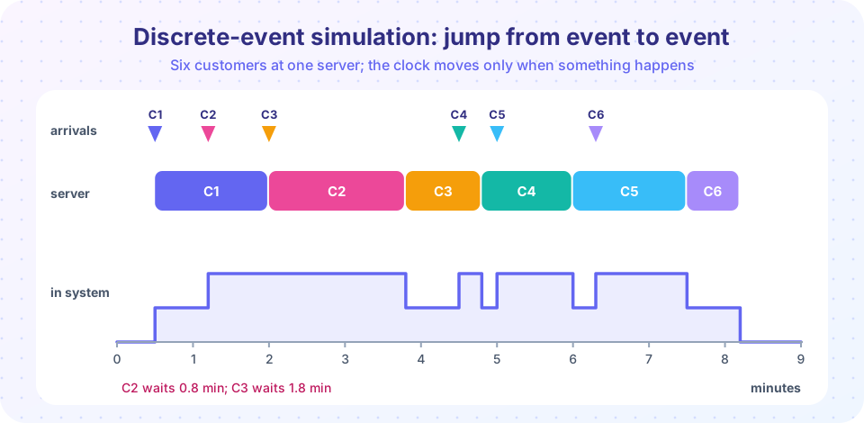
A discrete-event simulation keeps a clock and an event list. At each step it removes the earliest event, moves the clock to that event's time, updates the state and schedules any new events it causes. In a queue only two kinds of event matter:
- Arrival at time
t: schedule the next arrival. If a server is free, the customer starts service and a departure is scheduled att + (a random service time). Otherwise the customer joins the line. - Departure at time
t: if someone is waiting, the first in line starts service now (a new departure is scheduled). Otherwise, one server becomes free.
Nothing happens between events, so the clock simply leaps forward. A simulation can cover a year of a busy hospital in seconds, because only the events cost time.
Randomness comes from a pseudo-random number generator that produces numbers that look random but follow a fixed sequence from a starting seed. Using the same seed reproduces the same run, which is essential for debugging and for fair comparisons.
Try it: an event-driven simulator
The code below is a complete simulator for an M/M/c queue. The event list is a Python heap (a priority queue) that always yields the earliest event. We test it on the help-line from the last lesson, where Erlang C predicts an average wait of 21.07 minutes with three agents.
Press Run (or Ctrl + Enter) to see the result here.
Program input · what you'd type while the program runs
Type the answers before you press Run, one per line. Each time the program reads a line (with input()), it gets the next line from this box.
The simulated numbers should land close to the theoretical ones. That is the first test of any simulator: validation, running a case where you know the answer. Once validated, you can change the rules (add priorities, breaks or limited waiting space) and trust the results more.
One run is not an answer
Each run is a random sample. Two runs with different seeds give different averages, so you must report how much they vary. The standard method:
- Run
nindependent replications (different seeds). - Take the average result of each, then the mean
x̄and standard deviationsof those averages. - Report a 95 percent confidence interval:
x̄ ± t · s / √n, wheret ≈ 2.05for 30 replications.
The interval says: if you repeated the whole experiment many times, about 95 percent of such intervals would cover the true long-run mean. More replications make it narrower.
The warm-up problem
Simulations usually start with an empty system, and that is not typical. The first customers find no line, so the early waits are too short. If you average everything, your estimate is biased low. The fix is to discard an initial warm-up period (or to start from a typical state). Plot the running average over time to see where it settles.
Press Run (or Ctrl + Enter) to see the result here.
Program input · what you'd type while the program runs
Type the answers before you press Run, one per line. Each time the program reads a line (with input()), it gets the next line from this box.
The first 100 customers wait much less than the long-run figure, which is why the warm-up must go. The interval should cover the theoretical 48 minutes in most runs of this experiment, but about 1 time in 20 it will not, and that is exactly what "95 percent" means.
Why simulate? A question formulas cannot answer
The M/M/1 formulas assume exponential service times. Suppose the real service takes almost exactly the same time every time, say 12 minutes. Then the formula must be replaced by the Pollaczek-Khinchine formula for an M/G/1 queue, or we can just change one line in the simulator. Using the clinic numbers λ = 4 and μ = 5 per hour:
Press Run (or Ctrl + Enter) to see the result here.
Program input · what you'd type while the program runs
Type the answers before you press Run, one per line. Each time the program reads a line (with input()), it gets the next line from this box.
All three systems have the same arrival rate and the same mean service time, and the same utilization of 0.8, yet their waits differ greatly. Variability itself costs time. This is a principle worth remembering: reducing variation in service often helps as much as adding capacity.
Good simulation practice
- Validate against a formula or real data before trusting new scenarios.
- Use separate random streams for arrivals and service so that changes in one do not alter the other. With the same seeds across scenarios (common random numbers), differences between options are less noisy.
- Report intervals, not single numbers.
- State your assumptions: input distributions should come from data, not from convenience.
Choosing the inputs
A simulation is only as good as its inputs. Where do the interarrival and service-time distributions come from? Ideally from data: record timestamps, then look at histograms and compute means and standard deviations. If the data look exponential, use the exponential; if service times are nearly constant with a little noise, a shifted or gamma distribution may fit better. When no data exist, use expert estimates such as the minimum, most likely and maximum values (a triangular distribution), and note this in the report as an assumption.
Also keep random number streams separate: draw arrivals from one generator and service times from another. Then changing one aspect of the model (say, adding a server) does not alter the sequence of arrivals, so two scenarios can be compared on exactly the same customers. This is the idea of common random numbers from the previous section, and it often reduces the number of replications needed to see a real difference between designs.
What can go wrong
- Bugs. A queue with one wrong comparison can silently produce plausible-looking nonsense. Validate against formulas and also check simple things by hand, such as the number of arrivals per hour.
- Too few replications. Report the interval; if it is wider than the difference you care about, run more.
- Non-steady behavior. If arrival rates change during the day, there is no steady state; measure what happens during the actual day, as the help-desk project in chapter 9 does.
- Over-modelling. Adding detail that does not change the answer costs time. Start simple and add realism only where it changes the decision.
Common misconceptions
"A simulation proves the answer." It gives an estimate with uncertainty. More replications narrow it, but they cannot fix a wrong model.
"The first run is representative." Empty-and-idle starts bias the results; discard a warm-up.
"A longer run replaces replications." Long runs help, but independent replications give you an honest measure of variability.
Check your understanding
Quick check · 5 questions
of 5 answered You scored / 5 · perfect!
-
1. What does the event list contain?
The simulator repeatedly takes the earliest scheduled event and advances the clock to its time. -
2. Why discard a warm-up period?
The initial empty state biases the averages, so early observations are dropped to estimate steady-state behavior. -
3. 30 replications give a mean of 50 minutes, a standard deviation of 6 and t = 2.05. What is the half-width of the 95% interval?
Half-width = 2.05 × 6 / √30 ≈ 2.2 minutes. -
4. Why do constant service times produce shorter lines than exponential ones with the same mean?
Waiting is driven by variability as well as by the average load. -
5. Using the same seed reproduces what?
A pseudo-random generator is deterministic, so a seed fixes the whole sequence.
Summary
- A discrete-event simulation keeps a state, a clock and an event list, and jumps from event to event.
- Validate a simulator on a case with a known answer before using it on new questions.
- Use replications, discard a warm-up period and report confidence intervals.
- Service variability changes waiting times even when the average and the utilization are unchanged.
Next: Chapter 6 review
Track your progress
Create a free account to tick off lessons and pick up where you left off on any device.
of Operations Research lessons completed