


















Lesson 44 of 49 · Projects and Practice
Project: Test an Inventory Policy by Simulation
Build a daily inventory simulator with random demand and delivery delay, compare it with EOQ and safety-stock formulas, and search for the cheapest reorder policy.
In chapter 5 you learned formulas for the order quantity and the reorder point. They assume simple things, such as constant lead times, and they treat the quantity and the timing as separate questions. In this project you will build a simulator that plays out years of a warehouse, day by day, count what each policy really costs, and compare the result with the formulas. This is how practitioners check formulas before trusting them, and how they investigate situations the formulas do not cover.
What you will learn
- How to turn an inventory policy into a day-by-day simulation.
- How to compare simulated costs with EOQ and reorder-point formulas.
- How to search for the best policy and read the result as a trade-off.
- How to test a policy against changes in the assumptions.
Key terms
Inventory position: stock on hand plus stock already ordered but not yet received.
(r, Q) policy: whenever the inventory position falls to or below r (the reorder point), order Q units.
Lost sales: demand that cannot be served from stock and disappears.
Fill rate: the fraction of demand served from stock.
Common random numbers: using the same random demand stream for every policy tested, so differences reflect the policy and not luck.
The problem
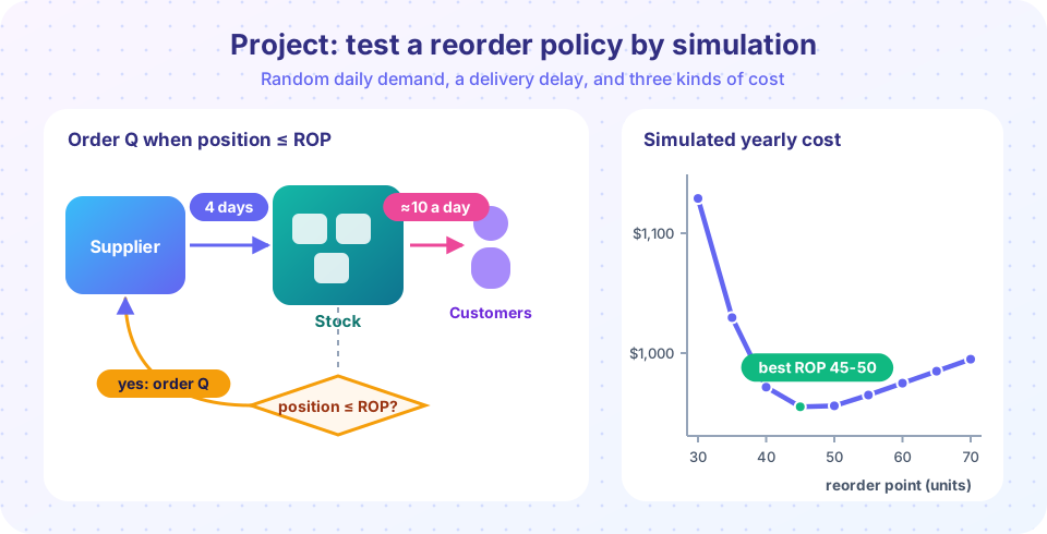
A shop sells about 10 units a day (3,650 a year) of a product. Daily demand is random with a Poisson distribution (mean 10, standard deviation about 3.2). The supplier delivers exactly 4 days after an order. The costs (example figures) are:
| Cost | Value |
|---|---|
| Fixed cost per order | $60 |
| Holding cost | $2 per unit per year |
| Lost sale | $5 per unit not served |
Task: choose the order quantity Q and the reorder point r to minimize the total yearly cost.
Step 1: What the formulas suggest
- EOQ:
Q = √(2 × 3,650 × 60 / 2) ≈ 468. - Demand during the 4-day lead time has mean
4 × 10 = 40and standard deviation√40 ≈ 6.3. - A 95 percent cycle service level adds
1.645 × 6.3 ≈ 10.4units of safety stock, sor ≈ 40 + 10.4 ≈ 50.
So the formulas say: order 468 whenever the inventory position reaches about 50.
Step 2: The simulator
Each simulated day, in this order: receive any delivery due today, serve demand from stock (lost sales if stock is short), add the day's holding cost, and then check the inventory position against r. If it is at or below r, place an order that will arrive after the lead time.
Press Run (or Ctrl + Enter) to see the result here.
Program input · what you'd type while the program runs
Type the answers before you press Run, one per line. Each time the program reads a line (with input()), it gets the next line from this box.
Read the table from the top: at a reorder point of 30 the shop often runs dry during the lead time and the lost-sales bill is large. As the reorder point rises, lost sales fall quickly and holding cost rises slowly. The cheapest point is near 45 to 50, which agrees with the formula's suggestion of about 50. The curve is also flat: moving the reorder point by 5 units around the minimum changes the yearly cost by only a few dollars, which echoes the flat EOQ cost curve you met in chapter 5.
Step 3: Search both decisions together
The formulas treat Q and r separately, but they interact: a larger Q means fewer orders and therefore fewer chances to run out. A small grid search over both uses the same simulator.
Press Run (or Ctrl + Enter) to see the result here.
Program input · what you'd type while the program runs
Type the answers before you press Run, one per line. Each time the program reads a line (with input()), it gets the next line from this box.
The best cell sits near the EOQ and the formula-based reorder point, and neighboring cells are close in cost. Remember that each number is a simulated average, so differences of a few dollars are within the noise of the simulation. This is a good reason to use common random numbers: every policy here sees the same demand streams.
Step 4: Stress-test the assumption of a fixed lead time
Real suppliers are not exactly on time. Suppose the lead time is random, from 2 to 6 days with equal chances (mean 4, the same as before). The formulas that assumed a fixed 4 days no longer apply. The simulator can handle it by changing one line.
Press Run (or Ctrl + Enter) to see the result here.
Program input · what you'd type while the program runs
Type the answers before you press Run, one per line. Each time the program reads a line (with input()), it gets the next line from this box.
With random lead times the cheapest reorder point moves up, from about 50 to about 60, and the best cost rises from roughly $954 to roughly $988 a year: unreliable delivery is paid for with extra safety stock. A supplier who delivers reliably in 4 days is worth more than one who delivers in 4 days on average. This kind of question is exactly what simulation is for.
What to put in your report
- The problem and the numbers, including which are assumptions (demand pattern, costs).
- The formula answer and the simulated answer, with the observation that they agree within noise.
- A sensitivity statement: cost is flat near the optimum, but rises with lead-time variability.
- A recommendation: for instance, order about 470 units when the position is at or below about 50, and monitor the fill rate; talk to the supplier about reliability.
- Limitations: demand assumed stationary and Poisson, no seasonality, a single product.
Extensions to try
- Replace Poisson demand by a seasonal pattern and see whether a single reorder point still works.
- Add a quantity discount from chapter 5 and re-optimize.
- Switch lost sales to backorders (the customer waits; a smaller penalty).
- Compare against a periodic-review policy that orders every 7 days up to a target level.
How to read the results
The sweep tells a clear story. At small reorder points the yearly cost is dominated by lost sales; at large ones, by holding cost. The minimum is flat, so a reorder point anywhere in a band around 45 to 55 is nearly as good as the best, and the choice among them can be made on other grounds, such as the risk that a customer is disappointed. If management cares about a fill rate of at least 99.9 percent, the table shows that a reorder point of 45 or more is needed, and the cheapest point (45) already meets that target. That is how a cost model and a service target are combined: first find the cost curve, then choose the cheapest point that meets the target.
Be careful about reading small differences. Each cost is an average over five simulated demand streams of ten years each, so a difference of a few dollars is within the simulation noise. When two policies are that close, treat them as equal and decide by other criteria.
Presenting the project
Executives rarely want to see code. A one-page summary works well: the policy (order about 470 units when the position reaches about 50), its expected cost, the fill rate, a chart of the cost against the reorder point showing the flat bottom, and the sensitivity to lead-time variability. Add one sentence about what you would do next, for example collecting a year of actual delivery times to replace the assumed distribution.
Common misconceptions
"The simulation's best cell is the true optimum." It is the best on a coarse grid with random noise. Use it to find the neighborhood of good policies, not an exact point.
"Formulas make simulation unnecessary." Formulas are the starting point and the check; simulation handles the rules the formulas cannot.
Check your understanding
Quick check · 5 questions
of 5 answered You scored / 5 · perfect!
-
1. What is the inventory position?
The reorder rule uses the position so that an outstanding order is not forgotten and a second order placed too early. -
2. Why use the same random demand streams for all policies?
Common random numbers reduce noise when comparing alternatives. -
3. Which cost rises when the reorder point is raised?
A higher reorder point means more safety stock, which costs more to hold but reduces lost sales. -
4. Delivery times vary around the same average. What usually happens to the best reorder point?
More variability in the lead time needs more safety stock to keep the same service. -
5. Demand mean 10 per day, lead time 4 days, safety stock 10. What is the reorder point?
ROP = mean lead-time demand + safety stock = 40 + 10 = 50.
Summary
- A day-by-day simulator turns an inventory policy into a measurable cost.
- The simulation agrees with the EOQ and reorder-point formulas, and shows a flat cost near the best policy.
- Common random numbers make comparisons fair.
- Changing assumptions (random lead time) is cheap in a simulation, and shows what reliability is worth.
Track your progress
Create a free account to tick off lessons and pick up where you left off on any device.
of Operations Research lessons completed