


















Lesson 19 of 49 · Network Optimization
Shortest Paths and Dijkstra's Algorithm
Learn how Dijkstra's algorithm finds shortest paths, trace it by hand on a delivery network, code it with a heap and check it against scipy and an LP model.
How do you get from the depot to a customer using the least distance, time or money? This is the shortest path problem, probably the most familiar network problem: every navigation app solves it millions of times a day. The edge weights can be kilometers, minutes, tolls or even risks. In 1956 the Dutch computer scientist Edsger W. Dijkstra designed an elegant algorithm for it (published in 1959), and a refined form of it is still at the heart of routing software.
In this lesson you trace Dijkstra's algorithm by hand, write it in Python, and verify it two other ways.
What you will learn
- The shortest path problem and its variants.
- Dijkstra's algorithm: tentative and settled distances.
- How to reconstruct the route from predecessor labels.
- Why the algorithm needs nonnegative weights, and what to use otherwise.
Key terms
Shortest path: a path whose edge weights add to the smallest possible total.
Tentative distance: the best distance found so far to a node; it may still improve.
Settled node: a node whose shortest distance is final.
Relaxation: checking whether going through a node gives a shorter route to a neighbour, and updating if so.
Predecessor: the node just before this one on its shortest path; following predecessors backwards gives the route.
The problem and its variants
Given a network with nonnegative edge weights and a start node s:
- Single-pair: find the shortest path from
sto one targett. - Single-source: find shortest paths from
sto every other node. Dijkstra's algorithm solves this version, and often does not cost more than the single-pair case. - All-pairs: find shortest distances between every pair of nodes (Floyd–Warshall or repeated Dijkstra).
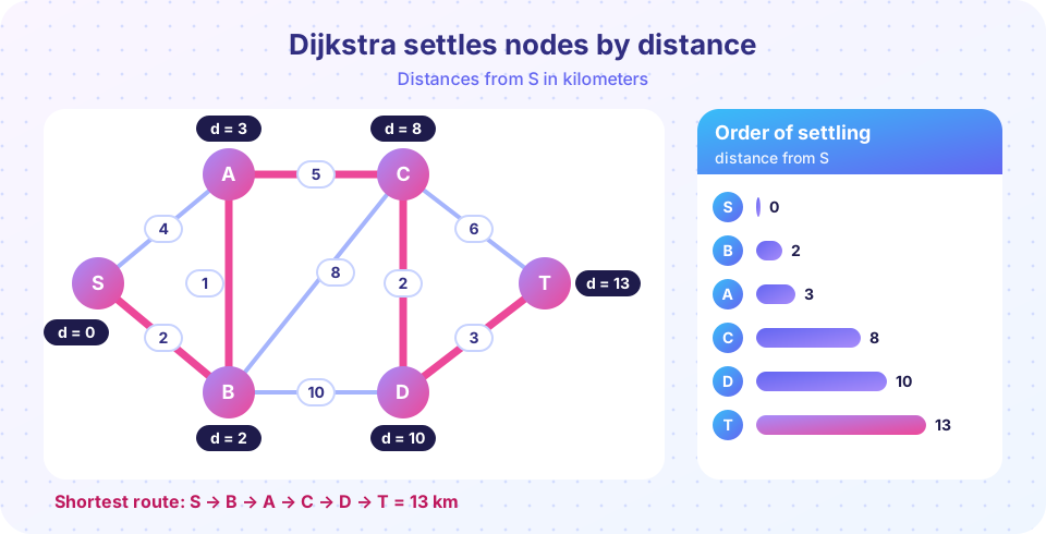
Our example network has depot S, towns A, B, C, D and customer T, with these road lengths in kilometers (example numbers): S–A 4, S–B 2, A–B 1, A–C 5, B–C 8, B–D 10, C–D 2, C–T 6, D–T 3.
The idea of Dijkstra's algorithm
Keep, for every node, a tentative distance from S. Start with 0 for S and infinity for everyone else. Then repeat:
- Among nodes not yet settled, pick the one with the smallest tentative distance. Its distance is now final: settle it.
- Relax the edges leaving it: for each neighbour, if "distance to this node + edge weight" is smaller than the neighbour's tentative distance, update the neighbour (and remember this node as its predecessor).
- Stop when the target (or every node) is settled.
Why is the smallest tentative distance already final? Every other unsettled node is at least as far away, and weights are not negative, so any route through those nodes can only be longer. This is a greedy argument, and it is exactly why negative weights break the method.
Worked example
| Step | Settle | S | A | B | C | D | T |
|---|---|---|---|---|---|---|---|
| start | 0 | ∞ | ∞ | ∞ | ∞ | ∞ | |
| 1 | S (0) | 0 | 4 | 2 | ∞ | ∞ | ∞ |
| 2 | B (2) | 0 | 3 | 2 | 10 | 12 | ∞ |
| 3 | A (3) | 0 | 3 | 2 | 8 | 12 | ∞ |
| 4 | C (8) | 0 | 3 | 2 | 8 | 10 | 14 |
| 5 | D (10) | 0 | 3 | 2 | 8 | 10 | 13 |
| 6 | T (13) | 0 | 3 | 2 | 8 | 10 | 13 |
Bold numbers show where relaxation improved a value. At step 2, going S → B → A costs 2 + 1 = 3, which beats the direct road S → A (4). At step 3, A → C gives 3 + 5 = 8, better than B → C (2 + 8 = 10). At step 4, C → D gives 8 + 2 = 10, better than B → D (2 + 10 = 12), and at step 5, D → T gives 10 + 3 = 13, better than C → T (8 + 6 = 14).
To find the route, follow predecessors backwards from T: T ← D ← C ← A ← B ← S. The route is S → B → A → C → D → T, 13 km.
Dijkstra in Python
A priority queue (a heap) hands you the unsettled node with the smallest tentative distance quickly. Python's heapq provides one.
Press Run (or Ctrl + Enter) to see the result here.
Program input · what you'd type while the program runs
Type the answers before you press Run, one per line. Each time the program reads a line (with input()), it gets the next line from this box.
Compare the printed "improve" lines with the bold numbers in the table: they match.
Dijkstra with scipy
For real work you call a library. scipy.sparse.csgraph.dijkstra takes the adjacency matrix and can also return predecessors. The block below also draws the distances.
Press Run (or Ctrl + Enter) to see the result here.
Program input · what you'd type while the program runs
Type the answers before you press Run, one per line. Each time the program reads a line (with input()), it gets the next line from this box.
Shortest path as a linear program
Remember that network problems are linear programs. Send one unit of "flow" from S to T. Let x_uv be the amount of flow on arc u → v (we make each road a pair of arcs). Then:
minimize   Σ weight(u,v) · x_uv
subject to flow out of S − flow into S = 1
           flow out of T − flow into T = −1
           flow out − flow in = 0         for every other node
           x ≥ 0
The constraints say: one unit leaves S, one unit arrives at T, and every intermediate node passes on what it receives. The cheapest way to move the unit is the shortest path, and because of total unimodularity the optimal x consists of zeros and ones along the route.
Press Run (or Ctrl + Enter) to see the result here.
Program input · what you'd type while the program runs
Type the answers before you press Run, one per line. Each time the program reads a line (with input()), it gets the next line from this box.
The LP agrees with Dijkstra: 13 km along the same arcs. Dijkstra is much faster, but the LP view is useful because you can add side constraints (for example "at most 3 tolls") that destroy the pure shortest-path structure.
Efficiency and limits
With a simple array, Dijkstra takes about n² steps for n nodes. With a binary heap it takes about (n + m) log n steps for m edges, fast enough for road networks with millions of edges when combined with clever pre-computation. Practical navigation systems also use goal-directed variants such as A*, which uses an estimate of the remaining distance to avoid exploring nodes in the wrong direction.
Negative weights break Dijkstra's greedy argument. If some edges have negative weights (for example a refund for taking a certain route), use the Bellman–Ford algorithm, which relaxes all edges repeatedly and also detects negative cycles. A negative cycle makes "shortest path" meaningless, since you could go around forever to lower the cost.
Common misconceptions
"The path with the fewest edges is the shortest." In a weighted network the shortest route may use more, but lighter, edges. Here S → B → A → C → D → T has five edges while S → A → C → T has three but is longer (15 km).
"Dijkstra's algorithm can handle negative weights." It cannot; use Bellman–Ford.
"Once a node has a tentative distance, it is final." Only settled nodes are final; tentative values can still improve.
Check your understanding
Quick check · 5 questions
of 5 answered You scored / 5 · perfect!
-
1. Which node does Dijkstra's algorithm settle next?
With nonnegative weights, the closest unsettled node cannot be reached more cheaply through others. -
2. In the worked example, why does A's distance fall from 4 to 3?
Relaxation found a cheaper route through B. -
3. What is the length of the shortest route from S to T in the example network?
S → B → A → C → D → T has length 2 + 1 + 5 + 2 + 3 = 13. -
4. Which algorithm handles negative edge weights (without negative cycles)?
Bellman–Ford relaxes all edges repeatedly and works with negative weights. -
5. How do you recover the route after running Dijkstra?
Each node stores the node from which its best distance came.
Summary
- The shortest path problem finds the minimum-weight route; Dijkstra's algorithm solves it for nonnegative weights.
- It repeatedly settles the unsettled node with the smallest tentative distance and relaxes its edges.
- Predecessor labels give the route; the example route is S, B, A, C, D, T with length 13 km.
- A heap makes it fast;
scipy.sparse.csgraph.dijkstraprovides it ready-made. - Negative weights need Bellman–Ford; the problem can also be written as a small LP.
Next: Minimum Spanning Trees
Track your progress
Create a free account to tick off lessons and pick up where you left off on any device.
of Operations Research lessons completed