


















Lesson 25 of 49 · Inventory and Scheduling
The EOQ Model: How Much to Order
Derive and use the economic order quantity formula, find the best order size, reorder point and yearly cost, and see why the answer is forgiving.
In 1913 an engineer named Ford W. Harris published a short paper asking a plain question: how many parts should a factory make in one batch? His answer, later popularized by R. H. Wilson, became the economic order quantity (EOQ). More than a century later it is still the first model every inventory course teaches, because it captures the central trade-off in one tidy formula and because its logic reaches far beyond its assumptions.
This lesson builds the model from scratch, derives the formula without any calculus-heavy detours, and then tests how much the answer matters when your numbers are a little off.
What you will learn
- The assumptions of the EOQ model and what each one means.
- How to write yearly ordering, holding and total cost as functions of the order quantity Q.
- How to derive and apply
Q* = √(2DS / H), and to find the cycle length and the reorder point. - Why the total cost is flat near the optimum, and what that means in practice.
Key terms
D: demand per year, in units.
S: fixed cost of placing one order, in dollars.
H: holding cost per unit per year, in dollars (often a percentage of the item's value).
Q: order quantity, the number of units in each order. Q* is the best value.
Reorder point (ROP): the stock level at which a new order is placed so that it arrives just as stock reaches zero.
The assumptions
The basic EOQ model rests on a short list of simplifications. Knowing them is part of using the model well.
- Demand is known and constant, at
Dunits per year. - Each order costs a fixed
Sregardless of its size. - Holding one unit costs
Hper year, proportional to time on the shelf. - Lead time is known and constant, and the order arrives all at once.
- Shortages are not allowed, and prices do not depend on the order size.
Under these assumptions, stock follows a clean sawtooth: an order of Q units arrives, demand drains it at a steady rate until it reaches zero, and the next order lands at that exact moment. The stock averages Q/2 over a cycle, because it falls in a straight line from Q to 0.
Building the cost function
Over one year:
- The number of orders is
D / Q, so the ordering cost isS × D / Q. - The average stock is
Q / 2, so the holding cost isH × Q / 2. - The purchase cost
D × pricedoes not depend onQin this model, so we leave it out of the comparison.
The total relevant cost is
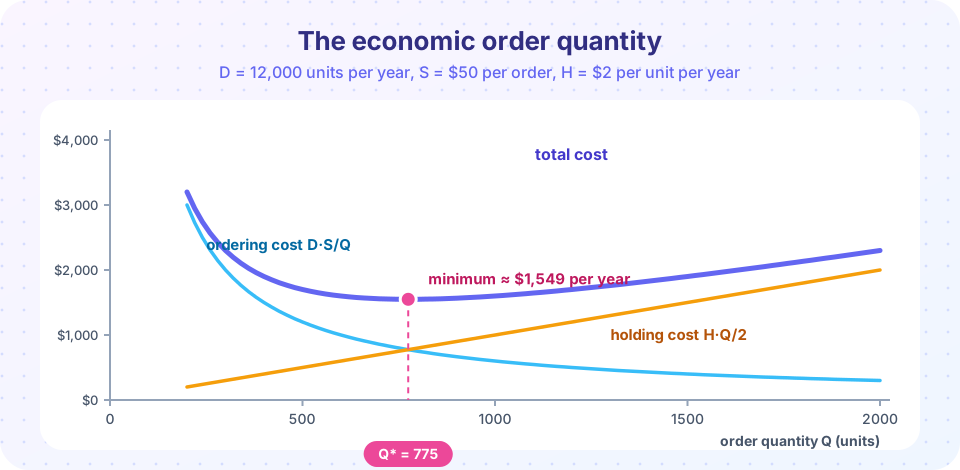
TC(Q) = D·S / Q + H·Q / 2
The first term shrinks as Q grows; the second grows. Their sum is a U-shaped curve with a single lowest point.
Finding the minimum
Calculus gives the answer in one line: set the derivative dTC/dQ = −D·S / Q² + H / 2 equal to zero, which gives Q² = 2DS / H. You can also see it without calculus. For this U-shaped sum, the minimum happens where the two terms are equal: D·S / Q = H·Q / 2. Solving for Q gives the same result:
Q* = √(2DS / H)
At the optimum, ordering cost and holding cost are exactly equal, and the minimum total cost is TC* = √(2DSH).
A worked example
A small pharmacy sells 12,000 boxes of a vitamin each year. Each order costs $50 to place and process, and holding one box for a year costs $2.
Q* = √(2 × 12,000 × 50 / 2) = √600,000 ≈ 774.6, so order about 775 boxes.- Orders per year:
12,000 / 774.6 ≈ 15.5. - Cycle length:
365 / 15.5 ≈ 23.6days between orders. - Minimum yearly cost:
√(2 × 12,000 × 50 × 2) = √2,400,000 ≈ $1,549, split evenly: about $775 for ordering and $775 for holding.
The reorder point
Suppose the supplier needs 5 days to deliver. Daily demand is 12,000 / 365 ≈ 32.9 boxes, so during the lead time customers buy about 164 boxes. The pharmacy should place the next order when stock falls to the reorder point:
ROP = daily demand × lead time ≈ 32.9 × 5 ≈ 164 boxes
Note that the reorder point depends on demand and lead time, not on Q. The two decisions, how much and when, are separate in this model.
Try it
First, a live calculator. Move the slider and watch the two costs trade places.
Now compute the formula and compare it with a brute-force search over all order sizes, which proves the formula really is the minimum.
Press Run (or Ctrl + Enter) to see the result here.
Program input · what you'd type while the program runs
Type the answers before you press Run, one per line. Each time the program reads a line (with input()), it gets the next line from this box.
How forgiving is the answer?
Real inputs are estimates. What if the demand forecast or the holding cost is wrong, so that you order the wrong amount? A neat identity shows the penalty. If r = Q / Q*, then
TC(Q) / TC* = (r + 1/r) / 2
Ordering 50 percent too much (r = 1.5) costs (1.5 + 0.667) / 2 = 1.083, only 8.3 percent above the minimum. Ordering twice the optimum costs 25 percent more. Ordering half costs the same 25 percent more. The curve is wide and flat near the bottom, so a rounded, convenient quantity such as a full pallet is nearly as good as the exact optimum.
A second consequence concerns the inputs. Because Q* involves a square root, a 21 percent error in D·S / H changes Q* by only 10 percent. Mistakes in the cost estimates are damped.
Press Run (or Ctrl + Enter) to see the result here.
Program input · what you'd type while the program runs
Type the answers before you press Run, one per line. Each time the program reads a line (with input()), it gets the next line from this box.
Why a square root?
The square root in Q* = √(2DS/H) is not a quirk of algebra; it follows from balance. Suppose ordering gets twice as expensive (S doubles). You would like to order bigger batches to place fewer orders, but bigger batches raise the holding bill, which pushes back. The two effects compromise at a batch that is only √2 ≈ 1.41 times larger, not twice as large. In the pharmacy example, doubling S from $50 to $100 moves the best order from 775 boxes to about 1,095 and raises the yearly cost from $1,549 to about $2,191, which is again a factor of √2. Because the same root appears in the minimum cost √(2DSH), every input is damped: a 10 percent error in D, S or H changes the cost by about 5 percent at most.
Real-world adjustments
Managers rarely order the exact EOQ. Suppliers sell in cartons or pallets, so the quantity is rounded to a multiple of the pack size. Suppliers may require a minimum order or offer a discount above a threshold (the next lesson). Storage space may cap the batch. Because the cost curve is flat, these adjustments usually cost little. Where they matter, add them as constraints: compute the EOQ first as a benchmark, then evaluate the cost of the nearest feasible quantities and take the cheapest. This "benchmark, then adjust" habit is typical of practice: the formula gives you a target and tells you how much a deviation costs.
Common misconceptions
"The EOQ must be an exact whole number of units." The curve is so flat that rounding to a convenient pack size changes the cost by a fraction of a percent.
"Place an order whenever stock is low." The EOQ fixes how much; the reorder point fixes when. Mixing them up produces orders that arrive too early or too late.
"Holding cost is just the warehouse rent." H includes the cost of money tied up in stock, insurance, handling, shrinkage and obsolescence. For many firms capital is the largest part, so H is often 15 to 30 percent of the item's value per year.
Check your understanding
Quick check · 5 questions
of 5 answered You scored / 5 · perfect!
-
1. At the EOQ, how do the yearly ordering cost and holding cost compare?
The total-cost curve is lowest where D·S/Q equals H·Q/2, so the two costs are equal at Q*. -
2. D = 9,000, S = $20 and H = $4. What is Q*?
Q* = √(2 × 9,000 × 20 / 4) = √90,000 = 300. -
3. Doubling the annual demand D changes Q* by what factor?
Q* is proportional to the square root of D, so doubling D multiplies Q* by √2. -
4. Daily demand is 40 units and lead time is 6 days. What is the reorder point?
Demand during lead time is 40 × 6 = 240, so reorder when stock reaches 240. -
5. You order twice the EOQ. By how much does yearly relevant cost exceed the minimum?
With r = 2 the ratio is (2 + 0.5) / 2 = 1.25, so the cost is 25 percent above the minimum.
Summary
- EOQ assumes steady known demand, a fixed cost per order, linear holding cost and instant delivery.
- Total relevant cost is
D·S/Q + H·Q/2, minimized atQ* = √(2DS/H), where the two parts are equal. - The reorder point is demand during lead time and is decided separately from
Q*. - The cost curve is flat near the optimum, so rounded or slightly wrong quantities cost little.
Track your progress
Create a free account to tick off lessons and pick up where you left off on any device.
of Operations Research lessons completed