


















Lesson 36 of 49 · Decision Analysis and Game Theory
Decision Trees, Criteria and the Value of Information
Choose among alternatives under uncertainty with maximin, regret and expected value, roll back a decision tree, and compute the value of perfect and imperfect information.
A decision under uncertainty has a simple skeleton: alternatives, states of nature and payoffs. What is hard is deciding how to compare alternatives when the future is unknown. In this lesson you will learn several standard rules, see how they disagree, and then focus on the most widely used one, expected monetary value, together with the picture that makes it manageable: the decision tree. Finally you will learn to answer a question every manager asks: how much is a forecast, survey or test worth?
What you will learn
- How to apply maximin, maximax, Hurwicz, Laplace and minimax regret to a payoff table.
- How to compute expected monetary values and roll back a decision tree.
- How to calculate the expected value of perfect information (EVPI) and of an imperfect survey (EVSI).
- How to test how sensitive a decision is to the probabilities.
Key terms
Maximin: pick the alternative whose worst payoff is largest (pessimistic).
Maximax: pick the alternative whose best payoff is largest (optimistic).
Regret (opportunity loss): how much less you earn than the best alternative would have earned in that state.
EVPI: expected value of perfect information, the most a perfect forecast could be worth.
Posterior probability: a probability updated after seeing evidence, computed with Bayes' rule.
The payoff table and five rules
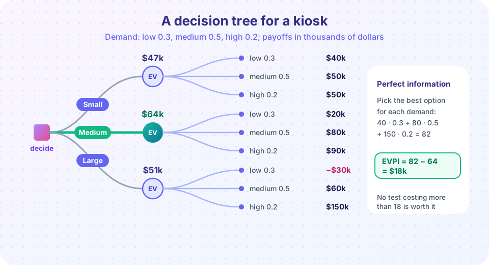
Return to the kiosk. Profit in thousands of dollars:
| Option | Low | Medium | High |
|---|---|---|---|
| Small | 40 | 50 | 50 |
| Medium | 20 | 80 | 90 |
| Large | −30 | 60 | 150 |
Without probabilities, you can apply attitude-based rules.
- Maximin (pessimist): worst cases are 40, 20 and −30, so choose Small.
- Maximax (optimist): best cases are 50, 90 and 150, so choose Large.
- Hurwicz with optimism index
α: score =α · best + (1 − α) · worst. Withα = 0.5the scores are 45, 55 and 60 (Large). - Laplace (treat states as equally likely): averages are 46.7, 63.3 and 60, so choose Medium.
- Minimax regret: in each state find the best payoff (40, 80, 150) and subtract. The regret table is Small 0, 30, 100; Medium 20, 0, 60; Large 70, 20, 0. The worst regrets are 100, 60, 70, so choose Medium.
Different attitudes give different answers, which is why a manager must say which attitude fits the situation. When probabilities are available, the standard approach is expected value.
Expected monetary value and the tree
With probabilities 0.3, 0.5 and 0.2, the expected value of each option is
- Small:
0.3 × 40 + 0.5 × 50 + 0.2 × 50 = 47 - Medium:
0.3 × 20 + 0.5 × 80 + 0.2 × 90 = 64 - Large:
0.3 × (−30) + 0.5 × 60 + 0.2 × 150 = 51
Medium has the highest EMV of $64k. A decision tree draws the same calculation. Work from the leaves back to the root (called rollback or backward induction):
- At a chance node, replace the node by the probability-weighted average of its branches.
- At a decision node, replace the node by the best branch.
Trees shine when decisions come in sequence, for example: first buy a survey, then choose a kiosk after seeing its result.
Press Run (or Ctrl + Enter) to see the result here.
Program input · what you'd type while the program runs
Type the answers before you press Run, one per line. Each time the program reads a line (with input()), it gets the next line from this box.
The value of perfect information
Suppose a clairvoyant could tell you the demand before you choose. You would pick Small if you hear "low" (40), Medium if "medium" (80), Large if "high" (150). The expected profit with perfect information is 0.3 × 40 + 0.5 × 80 + 0.2 × 150 = 82. Without information the best EMV is 64. The difference is the
EVPI = 82 − 64 = 18
An equal way to compute it is as the smallest expected regret: Medium's expected regret is 0.3 × 20 + 0.5 × 0 + 0.2 × 60 = 18. Either way, no source of information, however good, can be worth more than $18k to this decision. If a consultant wants $25k for a market study, the answer is already no.
Imperfect information: a survey
Real studies are imperfect. Suppose a survey reports "favorable" (F) or "unfavorable" (U), with these reliabilities: P(F | low) = 0.1, P(F | medium) = 0.6, P(F | high) = 0.9. Bayes' rule updates the probabilities:
P(F) = 0.3 × 0.1 + 0.5 × 0.6 + 0.2 × 0.9 = 0.51, soP(U) = 0.49.- After F, the posteriors are
P(low | F) = 0.03/0.51 ≈ 0.059,P(medium | F) ≈ 0.588andP(high | F) ≈ 0.353; after U, they shift toward low demand. - Choose the best kiosk for each result and average.
The expected profit with the survey minus 64 is the expected value of sample information (EVSI). It must lie between 0 and the EVPI.
Press Run (or Ctrl + Enter) to see the result here.
Program input · what you'd type while the program runs
Type the answers before you press Run, one per line. Each time the program reads a line (with input()), it gets the next line from this box.
The EVSI comes out at about 3.3 (thousand dollars), only a small share of the EVPI of 18, because the survey is a noisy signal. In general, 0 ≤ EVSI ≤ EVPI, and you should buy a study only if its price is below its EVSI.
Sensitivity: how sure must we be?
Probabilities are estimates. A decision is robust if small changes in them do not change the best choice. The plot varies the probability of high demand from 0 to 1, keeping the ratio low:medium at 3:5, and shows which alternative has the highest EMV.
Press Run (or Ctrl + Enter) to see the result here.
Program input · what you'd type while the program runs
Type the answers before you press Run, one per line. Each time the program reads a line (with input()), it gets the next line from this box.
The result is informative: Medium is best for any probability of high demand up to about 0.34, so the decision holds even if the estimate of 0.2 is off by a lot. If you believed high demand was 40 percent likely, the Large kiosk would win and more thought would be needed.
Utility and risk (a note)
EMV treats a gain of $100k and a loss of $100k as equal in size. Most people and firms are risk averse: losing the same money hurts more than winning it helps. The theory of utility (von Neumann and Morgenstern, 1944) replaces dollars by a utility function, usually concave, and maximizes expected utility. For small decisions in a large firm, EMV is a fine approximation. For a bet that could bankrupt you, it is not.
A sequential example: drill or sell?
A small mining company can sell its land now for $40k or drill at a cost of $25k. If it drills, there is a 30 percent chance of finding a deposit worth $150k and a 70 percent chance of finding nothing. The tree has a decision node (sell or drill) and a chance node after "drill". Rolling back: the chance node is worth 0.3 × 150 + 0.7 × 0 = 45, minus the drilling cost of 25 gives 20, which is less than the 40 from selling. So selling wins. Notice how little the numbers must change to alter the decision: if the deposit chance were 50 percent the drilling branch would be worth 75 − 25 = 50, above 40. The break-even chance is (40 + 25)/150 ≈ 0.43, which is exactly the kind of sensitivity statement a manager can use: "drill only if you believe the chance of success is above 43 percent".
A geologist's survey could shift that probability, and the EVSI machinery of this lesson tells you how much the survey is worth: it is only valuable if some possible result would change the decision.
Utility in one paragraph
If the company in this example has only $40k of capital, a failed $25k drilling would be a disaster, and the risk-neutral EMV rule would ignore that. Utility functions encode this by giving a loss a larger weight than an equal gain. In practice, analysts often keep EMV for routine decisions and use judgment, scenarios or simple utility curves for decisions where survival is at stake.
Common misconceptions
"The highest EMV is guaranteed to be best." It is best on average over many repetitions. In one play, you may get the bad outcome.
"Information is worth what it costs." It is worth at most its EVSI for imperfect and EVPI for perfect information. Pay only if the price is lower.
"Probabilities must be exact." They are judgments. Use sensitivity analysis to see whether the choice depends on them.
Check your understanding
Quick check · 5 questions
of 5 answered You scored / 5 · perfect!
-
1. Option X pays 10, 20, 30 and option Y pays 15, 18, 22 in three states. Which does maximin choose?
The worst cases are 10 for X and 15 for Y, and maximin picks the larger worst case. -
2. An option pays 100 with probability 0.4 and −20 with probability 0.6. What is its EMV?
0.4 × 100 + 0.6 × (−20) = 40 − 12 = 28. -
3. With perfect information the expected payoff is 90, and the best EMV without information is 72. What is the EVPI?
EVPI = 90 − 72 = 18. -
4. A consultant charges 25 for a study when EVPI is 18. What should you do?
No information can be worth more than 18, so a price of 25 is not justified even for a perfect study. -
5. In rolling back a tree, what do you do at a chance node?
At chance nodes you average the branch values by their probabilities; at decision nodes you take the best.
Summary
- Without probabilities, maximin, maximax, Hurwicz, Laplace and minimax regret encode different attitudes and can disagree.
- With probabilities, choose the highest EMV and compute it by rolling back a decision tree.
- EVPI is the expected payoff with perfect information minus the best EMV; no study can be worth more.
- Use Bayes' rule to value imperfect information (EVSI), and test sensitivity of the answer to the probabilities.
Next: Zero-sum games
Track your progress
Create a free account to tick off lessons and pick up where you left off on any device.
of Operations Research lessons completed