


















Lesson 29 of 49 · Inventory and Scheduling
Chapter 5 Review: Inventory and Scheduling
Review chapter 5 with a one-page picture, a table of formulas and rules, a quick calculator and a ten-question quiz on EOQ, EPQ, newsvendor and scheduling.
Chapter 5 gave you four families of tools. For steady demand you have the square-root models EOQ and EPQ. For random demand you have the critical ratio and safety stock. For ordering work you have SPT, EDD and Johnson's rule. This review puts them side by side so you can tell, for a new problem, which tool to reach for.
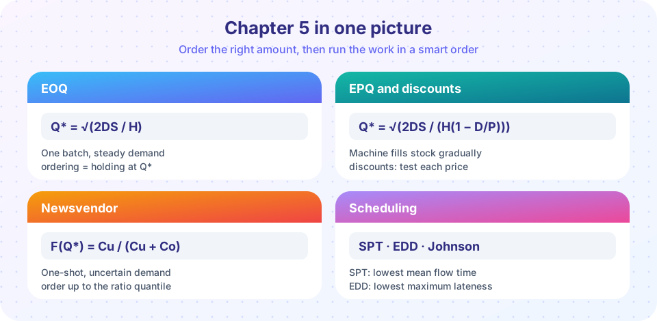
What you will learn
- To choose the right model from a problem description.
- To recall the key formulas and what each symbol means.
- To spot the assumptions behind each model and when they break.
The recap table
| Situation | Model | Key result | Watch out for |
|---|---|---|---|
| Steady demand, orders arrive at once | EOQ | Q* = √(2DS/H), TC* = √(2DSH) |
Ordering equals holding cost at the optimum |
| Steady demand, machine fills stock gradually | EPQ | Q* = √(2DS / (H(1 − D/P))) |
Peak stock is Q(1 − D/P) |
| Supplier price breaks | Discount EOQ | Clamp each level's EOQ, compare totals | Purchase cost must be included |
| One selling season, random demand | Newsvendor | F(Q*) = Cu/(Cu + Co) |
Mean demand is optimal only if Cu = Co |
| Repeated orders, random demand | Reorder point | ROP = mean lead-time demand + z·σ_L |
σ_L scales with √L |
| One machine, many jobs | SPT / EDD | SPT: average completion; EDD: maximum lateness | Different objectives, different rules |
| Two machines in series | Johnson | Ascending M1 for M1 ≤ M2, then descending M2 |
Optimal for two machines only |
A quick decision aid
The code below turns the first questions of that table into a small function. It is a study helper, not a full decision system.
Press Run (or Ctrl + Enter) to see the result here.
Program input · what you'd type while the program runs
Type the answers before you press Run, one per line. Each time the program reads a line (with input()), it gets the next line from this box.
Two mixed worked problems
Problem A. A store sells 3,600 items a year (use a 360-day year). Each order costs $45, and holding an item costs $1.50 per year. The lead time is 6 days. Find the order quantity, the number of orders, the cost and the reorder point (no safety stock).
Q* = √(2 × 3,600 × 45 / 1.5) = √216,000 ≈ 465items.- Orders per year:
3,600 / 465 ≈ 7.7, one every 46.5 days. - Yearly relevant cost:
√(2 × 3,600 × 45 × 1.5) = √486,000 ≈ $697. - Daily demand is 10, so the reorder point is
10 × 6 = 60items.
Problem B. Three jobs with times 5, 1 and 4 hours wait for one machine. SPT gives the order 1, 4, 5 with completion times 1, 5 and 10, a mean of 16/3 ≈ 5.33 hours. Any other order is worse: for example 5, 1, 4 gives completions 5, 6, 10 and a mean of 7.
Notice the habit in both: name the model, list the quantities with units, compute, and check that the result is plausible (the order quantity should be much smaller than a year's demand, and the SPT mean cannot exceed the total time of 10 hours).
How the exam questions hide the model
Questions rarely say "use EOQ". Look for the telltale phrases: "fixed cost per order and a holding cost per unit per year" means EOQ; "the machine produces while customers buy" means EPQ; "unsold items are salvaged at a loss" means newsvendor; "jobs wait for a machine and we want the smallest mean waiting time" means SPT; "two machines in series, minimize the finishing time" means Johnson.
Common misconceptions
"The formulas are laws." They are consequences of assumptions. If demand drifts, prices change daily or lead times vary, the formulas give a starting point, and simulation (chapter 6) checks it.
"Safety stock and the EOQ are the same decision." The EOQ sets order size; the reorder point and safety stock set order timing.
Check your understanding
Quick check · 10 questions
of 10 answered You scored / 10 · perfect!
-
1. D = 4,800, S = $75, H = $3. What is the EOQ?
Q* = √(2 × 4,800 × 75 / 3) = √240,000 ≈ 490. -
2. At the EOQ, which is true?
The total cost curve is lowest where the two components are equal. -
3. In the EPQ model with D/P = 0.5, how does the peak stock compare with the run size Q?
Peak stock = Q(1 − D/P) = 0.5 Q. -
4. Cu = $15 and Co = $5. What is the critical ratio?
15 / (15 + 5) = 0.75. -
5. Which statement about the reorder point is correct?
It covers expected demand during the wait plus a cushion for variability. -
6. Weekly demand has standard deviation 12 and lead time is 9 weeks (independent weeks). What is the lead-time standard deviation?
12 × √9 = 36. -
7. Which rule minimizes the mean completion time of jobs on one machine?
Shortest processing time first minimizes average completion time. -
8. Jobs on two machines: J1 (2, 7), J2 (6, 3), J3 (4, 4). Which order does Johnson's rule give?
J1 (2 ≤ 7) and J3 (4 ≤ 4) go first in ascending M1 order: J1, J3. J2 (6 > 3) goes last. -
9. Doubling D multiplies the EOQ by roughly...
Q* grows with the square root of D, and √2 ≈ 1.41. -
10. Which statement about a 95 percent cycle service level is correct?
The cycle service level counts cycles, not customers or units.
Summary
- EOQ and EPQ balance ordering (setup) cost against holding cost; EPQ scales holding by
1 − D/P. - Quantity discounts need the purchase cost and a feasibility check on each price level.
- The newsvendor critical ratio and the lead-time reorder point handle randomness.
- SPT, EDD and Johnson's rule are provably best for different scheduling objectives.
Track your progress
Create a free account to tick off lessons and pick up where you left off on any device.
of Operations Research lessons completed