


















Lesson 4 of 49 · Getting Started
A Python Toolkit for Operations Research
Meet the Python tools used throughout this course: scipy's linprog and milp, graph routines, numpy and matplotlib, with runnable bakery examples.
You can solve small OR models by hand, and you should, because that is how you learn what the algorithms do. But real problems have hundreds or thousands of variables, so you need software. This course uses Python because it is free, readable and runs in your browser on this site. You will not install anything: every code block has a Run button.
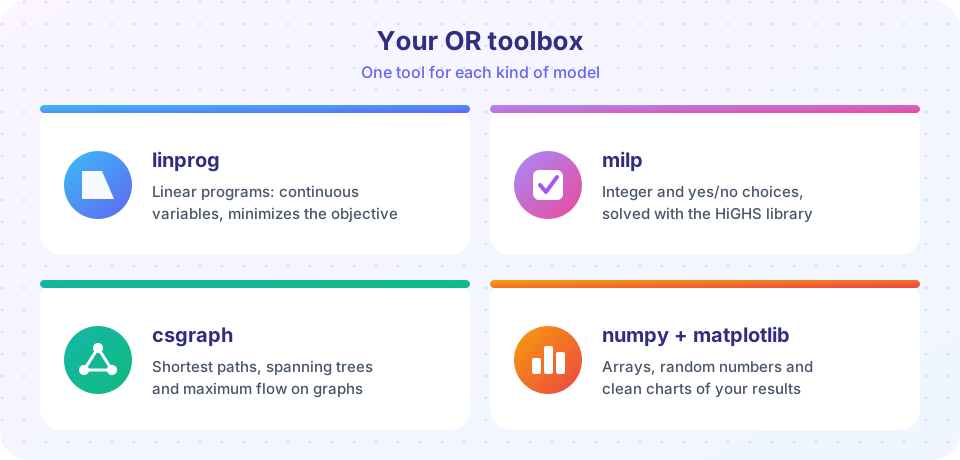
This lesson introduces the four pieces of the toolkit and solves the Sunrise Bakery problem with real solver code for the first time.
What you will learn
- How to read the inputs and outputs of
linprog. - How to add integer or yes/no variables with
milp. - Which graph routines are available for Chapter 4.
- How to draw a clean picture of a feasible region.
Key terms
Solver: software that finds an optimal solution to a model.
Feasible solution: a choice of values that satisfies every constraint.
Coefficient: a fixed number multiplying a variable, such as 60 in 60x.
Integrality: the requirement that a variable takes whole-number values.
Status: the solver's report of whether it succeeded, found the problem infeasible, or unbounded.
The four tools
| Tool | What it does | Used in |
|---|---|---|
scipy.optimize.linprog |
Solves linear programs with continuous variables | Chapters 2 and 3 |
scipy.optimize.milp |
Solves linear programs where some variables must be integers | Chapters 2, 3 and 5 |
scipy.sparse.csgraph |
Shortest paths, minimum spanning trees, maximum flow, matching | Chapter 4 |
numpy and matplotlib |
Arrays, simulation, random numbers and charts | everywhere |
Everything runs on top of the HiGHS solver, a fast open-source library for linear and mixed-integer programming. The code looks the same in a normal Python installation.
Solving a linear program with linprog
linprog always minimizes. To maximize profit, minimize its negative. The model
maximize   60x + 40y
subject to 2x +  y ≤ 16
            x + 2y ≤ 14
            x, y ≥ 0
becomes: cost vector c = [-60, -40], a matrix A_ub with one row per constraint, a right-hand side b_ub = [16, 14] and bounds of (0, None) for each variable (zero or more, no upper limit).
Press Run (or Ctrl + Enter) to see the result here.
Program input · what you'd type while the program runs
Type the answers before you press Run, one per line. Each time the program reads a line (with input()), it gets the next line from this box.
Read the output. status 0 means "optimal". The slack tells you how many hours of each resource are left over; a slack of zero means the resource is fully used, or binding. You will use that idea in the duality lesson of Chapter 3.
Possible statuses worth knowing: 2 means the problem is infeasible (no plan satisfies all constraints) and 3 means it is unbounded (the objective can improve forever, which usually signals a missing constraint).
Integers and yes/no choices with milp
Many decisions are whole numbers: you cannot build 2.5 warehouses. scipy.optimize.milp adds an integrality array: 1 for an integer variable, 0 for a continuous one. A binary variable is an integer variable between 0 and 1: a yes/no switch. The next example is a small project-selection problem: choose projects with the largest total value within a budget of 11 (in thousands of dollars).
Press Run (or Ctrl + Enter) to see the result here.
Program input · what you'd type while the program runs
Type the answers before you press Run, one per line. Each time the program reads a line (with input()), it gets the next line from this box.
Notice that the greedy idea "pick the biggest value first" would take project 1 (cost 7) and then project 3 (cost 4), a total value of 20, and miss a better combination. Integer programming checks combinations in a smart way; Chapter 3 shows how.
Graph tools for networks
Chapter 4 uses scipy.sparse.csgraph. A graph is stored as a matrix W where W[i][j] is the weight (distance, cost or capacity) of the arc from node i to node j. Functions such as dijkstra, minimum_spanning_tree and maximum_flow read this matrix. You will meet each one in its own lesson.
Drawing the feasible region
A feasible region is the set of all plans that obey the constraints. For two variables you can see it. The plot below marks every whole-number plan the bakery could consider, colors it by profit and circles the best one. Because the plot runs on this page, you can change the capacities and watch the region move.
Press Run (or Ctrl + Enter) to see the result here.
Program input · what you'd type while the program runs
Type the answers before you press Run, one per line. Each time the program reads a line (with input()), it gets the next line from this box.
From a written model to matrices
A solver wants numbers in rows and columns, so a skill you will use in every lesson is turning a constraint into one row of a matrix. Take the oven constraint 2x + y ≤ 16. Its coefficients, in the order of the variables (x, y), are [2, 1] and its right-hand side is 16. The baker constraint x + 2y ≤ 14 gives the row [1, 2] and the right-hand side 14. Stack the rows and you have A_ub = [[2, 1], [1, 2]] and b_ub = [16, 14]. If a constraint says "at least" (≥), multiply it by -1 to turn it into "at most", because linprog only accepts ≤ in A_ub. An equality constraint goes into the separate arguments A_eq and b_eq.
The order of the variables is a promise you make to yourself: the first column is always x, the second always y. Most beginner errors come from swapping a column or forgetting a sign, which is why the "verify by hand" habit below is worth the minute it takes.
Where the toolkit stops
These tools are exact for the problems they are built for, but each has limits. linprog cannot handle curved (nonlinear) objectives. milp can take a very long time on large integer problems, which is why Chapter 8 teaches heuristics. And none of them knows anything about your business: they will happily optimize a model with a wrong number in it. The toolkit gives you speed; judgment stays with you.
Habits that save time
- Name your data. Put numbers in lists with comments saying what they mean and which units they use.
- Check the status before trusting
res.x. An infeasible problem still returns numbers that mean nothing. - Verify by hand. Substitute the solution into every constraint yourself.
- Keep models small first. Test your formulation on two or three variables before scaling up.
A reliable workflow
When you meet a new problem, follow the same sequence every time and the code will almost write itself.
- Write the model in words and symbols first, on paper or in a comment.
- Put the data in named arrays (
profit,use,avail), with units in comments. - Call the solver and print the status before anything else.
- Print the solution next to the constraints and check each one, for example
use @ xagainstavail. - Plot or tabulate the result so that a human can judge it.
- Change one number and re-solve to see how stable the answer is.
This sequence is the modelling process of the previous lesson written as code, and it is the pattern behind every program in this course.
Common misconceptions
"The solver returns the true optimum of reality." It returns the optimum of your model. If a constraint is missing, the answer may be impossible in practice.
"Rounding a continuous solution gives the integer optimum." Rounding can break constraints or miss the best integer plan. Use milp or the methods of Chapter 3.
"linprog maximizes if I ask it to." It only minimizes. Negate the objective and negate the result.
Check your understanding
Quick check · 5 questions
of 5 answered You scored / 5 · perfect!
-
1. How do you maximize profit with linprog?
linprog only minimizes, so use c = -profit and report -res.fun. -
2. What does a slack of zero for a constraint mean?
Slack is unused resource. Zero slack means the limit is reached. -
3. Which function handles yes/no decisions?
milp supports integer variables; binary variables are integers bounded between 0 and 1. -
4. What does status 2 from linprog mean?
Status 2 means infeasible; status 3 is unbounded. -
5. Which module do the network algorithms of Chapter 4 come from?
csgraph provides shortest path, spanning tree and maximum flow routines.
Summary
linprogsolves linear programs (it minimizes),milpadds integer and binary variables,csgraphhandles networks.- Read
res.statusfirst, thenres.x,res.funand the slacks. - Binary variables model yes/no choices; rounding is not a safe substitute for integer programming.
- numpy and matplotlib build data and pictures; plotting the feasible region builds intuition.
- Always verify a solver's answer against the constraints by hand.
Next: Chapter 1 Review
Track your progress
Create a free account to tick off lessons and pick up where you left off on any device.
of Operations Research lessons completed