


















Lesson 10 of 49 · Modelling Decisions
Binary Variables and Logic in Models
Use yes/no variables to model selection, fixed setup costs, either-or rules and if-then conditions, with big-M constraints and milp examples.
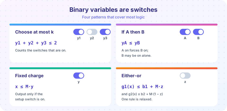
So far our variables could take any value in a range, which suits quantities such as hours and kilograms. But many real decisions are yes or no: open the warehouse or not, run the machine or not, fund the project or not. A binary variable is a variable that is either 0 or 1, and it is the key that opens a huge part of OR modelling. With binary variables you can express fixed costs, "choose at most two", "if A then also B" and many other rules that ordinary linear constraints cannot.
Models with binary or integer variables are called integer programs. They are harder to solve than linear programs, as Chapter 3 explains, but milp handles the small ones in this lesson in a blink.
What you will learn
- How a binary variable represents a yes/no decision.
- The standard formulas for "at most", "exactly", "if-then" and "not both".
- How a fixed setup cost is modelled with the big-M link
x ≤ M·y. - How to model an either-or rule, and why
Mshould be as small as possible.
Key terms
Binary variable: a variable restricted to 0 or 1; written y ∈ {0, 1}.
Fixed charge: a cost paid once if an activity is used at all, whatever its size.
Big-M constraint: a constraint using a large constant M to switch another constraint on or off.
Integer program (IP, MILP): an optimization model with integer variables; "mixed" means some variables are continuous.
Logical constraint: a linear inequality that expresses a rule such as "if A then B".
Selecting things: the pattern
Let yⱼ = 1 if project j is chosen and 0 otherwise. Choosing is then just a matter of adding up:
| Rule in words | Constraint |
|---|---|
| Choose at most 2 of the 4 projects | y₁ + y₂ + y₃ + y₄ ≤ 2 |
| Choose exactly 1 of the options | y₁ + y₂ + y₃ = 1 |
| Choose at least 1 | y₁ + y₂ + y₃ ≥ 1 |
| A and B cannot both be chosen | yₐ + y_b ≤ 1 |
| If A is chosen then B must be chosen (A requires B) | yₐ ≤ y_b |
| A is chosen exactly when B is | yₐ = y_b |
| Total cost within budget | Σ costⱼ · yⱼ ≤ budget |
Test them with the 4 combinations of 0 and 1. For yₐ ≤ y_b: (A=1, B=0) gives 1 ≤ 0, false, so that combination is forbidden; all three others are allowed. That matches "A requires B".
Example: a project portfolio
A company can fund four projects (example numbers, thousands of dollars):
| Project | A | B | C | D |
|---|---|---|---|---|
| Value | 50 | 40 | 45 | 25 |
| Cost | 60 | 40 | 30 | 20 |
The budget is 100. Funding project C only makes sense if project A is also funded (C builds on A), and management can run at most two projects at once.
Press Run (or Ctrl + Enter) to see the result here.
Program input · what you'd type while the program runs
Type the answers before you press Run, one per line. Each time the program reads a line (with input()), it gets the next line from this box.
The second row of the second call is the count limit and the third row is -a + c ≤ 0, that is c ≤ a. Without the logic, the best portfolio is B, C and D (value 110). With the rules in force, the best is A and C (value 95). The gap of 15 is the cost of the rules, which managers often want to know before they impose them.
Fixed charges and the big-M link
Often an activity has a setup cost that you pay once if you use it at all, no matter how much you produce. Cost is then no longer proportional to output, so a linear program cannot represent it directly. A binary variable y fixes this:
y = 1means "the activity is set up", and its fixed costFis paid: addF·yto the cost.- Output
xmay be positive only ify = 1: add the constraintx ≤ M·y.
If y = 0, then x ≤ 0, so output is zero. If y = 1, then x ≤ M, which is no restriction as long as M is at least the largest output you could ever make. M is the big-M, an upper bound on x. Pick it as small as the problem allows: oversized values of M make the solver's job harder.
Example: three products with setup costs
A workshop has 100 machine hours. Product data (example values):
| Product | Profit per unit | Hours per unit | Setup cost | Maximum demand |
|---|---|---|---|---|
| 1 | 12 | 2 | 200 | 50 |
| 2 | 9 | 1 | 500 | 60 |
| 3 | 7 | 1 | 50 | 80 |
If you ignore setups, the best plan fills the cheapest hours first: product 2 (9 per hour) up to 60 units, then product 3 with the remaining 40 hours. Profit before setups: 9·60 + 7·40 = 820. But that plan pays two setups, 500 and 50, so its real profit is only 270. Does a better plan exist?
Model: xⱼ units, yⱼ setup flags.
maximize   Σ profitⱼ·xⱼ − Σ setupⱼ·yⱼ
subject to Σ hoursⱼ·xⱼ ≤ 100
           xⱼ ≤ maxdemandⱼ · yⱼ        for each product
           xⱼ ≥ 0, yⱼ ∈ {0, 1}
Here the natural M for product j is its maximum demand.
Press Run (or Ctrl + Enter) to see the result here.
Program input · what you'd type while the program runs
Type the answers before you press Run, one per line. Each time the program reads a line (with input()), it gets the next line from this box.
The optimal plan sets up only product 3 and makes 80 units for a net profit of $510. The tempting plan that spreads hours over products 2 and 3 pays a setup cost of 500 for product 2 and nets only $270. Fixed charges change what is optimal, and a model that forgets them gives bad advice.
The picture of a fixed charge is a cost curve that jumps at zero:
Press Run (or Ctrl + Enter) to see the result here.
Program input · what you'd type while the program runs
Type the answers before you press Run, one per line. Each time the program reads a line (with input()), it gets the next line from this box.
Either-or constraints
Sometimes a rule says "constraint 1 or constraint 2 must hold, not necessarily both". Example: a machine runs either in mode 1 (2x + y ≤ 12) or in mode 2 (x + 3y ≤ 12). Use a binary z and a big M:
2x +  y ≤ 12 + M·z          (active when z = 0)
 x + 3y ≤ 12 + M·(1 − z)    (active when z = 1)
If z = 0, the first constraint is enforced while the second is relaxed by M, so it no longer bites. If z = 1, the roles swap. The solver chooses z to get the best objective. Again, take M just large enough that the relaxed constraint is never active.
A word on solver time
Each binary variable doubles the number of combinations the solver must reason about: 20 binaries give over a million combinations, and 100 give more than the number of grains of sand on Earth. The solver uses clever pruning (Chapter 3 introduces branch and bound), but models with tight formulations, small M values and few binaries solve far faster than loose ones.
A checklist for logical models
When you add binary variables, check the following before you solve.
- Name every binary clearly, for example
y_open[k] = 1 if warehouse k is open. - Test every logical constraint with all combinations of 0 and 1. Write a small truth table; it takes a minute and catches most sign errors.
- Choose each big-M from the data, such as the maximum demand or the capacity, never a round number like one million.
- Look at the cost of the rules. Solve once with and once without a logical rule and compare, as in the portfolio example.
Common misconceptions
"Use the largest M you can think of, to be safe." A huge M weakens the model and slows the solver, and numeric errors can appear. Choose the smallest valid bound.
"If-then needs a new kind of constraint." For binary variables yₐ ≤ y_b already says "if A then B".
"Rounding a continuous answer gives the right yes/no decision." Rounding setup variables often violates logic or costs; solve the integer model instead.
Check your understanding
Quick check · 5 questions
of 5 answered You scored / 5 · perfect!
-
1. Which constraint says "choose at most 3 of the 5 options" for binary variables y1..y5?
The sum of binary variables counts how many options are chosen, so ≤ 3 limits the count. -
2. Which constraint expresses "if A is chosen then B must be chosen"?
If yA = 1, then yB must be 1; if yA = 0, yB is free. -
3. In the fixed-charge link x ≤ M·y, what happens when y = 0?
With y = 0 the right side is 0, so x ≤ 0 and (with x ≥ 0) the output is zero. -
4. Why should M be as small as is valid?
Tight bounds give the solver a stronger formulation. -
5. The plan that ignores setups showed gross profit 820 but net 270 after paying two setups. What does this teach?
A model without the fixed charge optimizes the wrong objective.
Summary
- Binary variables model yes/no decisions; sums of them count what you choose.
- Use
≤,=and≥on sums for "at most", "exactly" and "at least";yₐ ≤ y_bmeans A requires B. - A fixed charge needs
F·yin the cost andx ≤ M·yas a link, withMas small as valid. - Either-or rules use a binary
zand big-M relaxation in both constraints. - Integer models are harder to solve; tight formulations help.
Next: Chapter 2 Review
Track your progress
Create a free account to tick off lessons and pick up where you left off on any device.
of Operations Research lessons completed