


















Lesson 14 of 49 · Linear and Integer Programming
The Simplex Method Step by Step
Learn how the simplex method walks from corner to corner using slack variables and a tableau, work the bakery example by hand and run a small simplex solver.
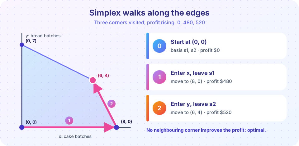
The graphical method needs a picture, and pictures stop at two or three variables. Real linear programs have thousands or millions of variables, so we need a procedure that works with numbers alone. That procedure is the simplex method, designed by George Dantzig in 1947. It starts at one corner of the feasible region, looks at the neighbouring corners, moves to one that improves the objective, and repeats until no neighbour is better. Because the optimum of an LP is always at a corner, the final corner is optimal.
In this lesson you will convert a model into the form the method needs, perform the pivots on the Sunrise Bakery problem by hand, and then run a small program that does the same thing.
What you will learn
- What slack variables are and why they turn inequalities into equations.
- How basic solutions correspond to corners of the feasible region.
- How to choose the entering variable, apply the ratio test and pivot.
- How to read the optimal plan and the shadow prices from the final tableau.
Key terms
Slack variable: a variable added to a ≤ constraint to measure the unused resource, turning it into an equation.
Basic variable: one of the variables allowed to be nonzero at the current corner; there is one per constraint.
Pivot: the row operation that swaps one variable into the basis and another out.
Entering variable: the nonbasic variable chosen to become basic because it improves the objective.
Ratio test: the rule that picks the leaving variable so that the next corner stays feasible.
Step 0: standard form with slack variables
Simplex works with equations. To convert 2x + y ≤ 16 into an equation, add a slack variable s₁ ≥ 0 that takes up the unused oven hours: 2x + y + s₁ = 16. Do the same with the baker constraint. The bakery model becomes:
maximize   60x + 40y
subject to 2x +  y + s₁       = 16
            x + 2y      + s₂  = 14
            x, y, s₁, s₂ ≥ 0
There are now 4 variables and 2 equations. A basic solution sets all but 2 variables (the nonbasic ones) to zero and solves for the other 2 (the basic ones). Each basic feasible solution is a corner of the region:
| Nonbasic (= 0) | Basic values | Corner |
|---|---|---|
x, y |
s₁ = 16, s₂ = 14 |
(0, 0) |
y, s₁ |
x = 8, s₂ = 6 |
(8, 0) |
s₁, s₂ |
x = 6, y = 4 |
(6, 4) |
x, s₂ |
y = 7, s₁ = 9 |
(0, 7) |
Setting a slack to zero means "this constraint is used up", so the corner lies on that constraint's line. Simplex moves between rows of this table by swapping one variable at a time.
The tableau
The tableau is a compact table of the equations plus a row for the objective. Write the objective as profit − 60x − 40y = 0, so the objective row holds −60, −40 under x and y.
| Basis | x | y | s₁ | s₂ | Right side |
|---|---|---|---|---|---|
| s₁ | 2 | 1 | 1 | 0 | 16 |
| s₂ | 1 | 2 | 0 | 1 | 14 |
| profit | −60 | −40 | 0 | 0 | 0 |
The current corner is x = y = 0, with s₁ = 16, s₂ = 14 and profit 0.
One iteration of simplex
- Optimality test. If every entry in the objective row is
≥ 0, stop: the current corner is optimal. - Entering variable. Otherwise pick a column with a negative entry in the objective row. The common rule (Dantzig's rule) takes the most negative one. Here that is
x(−60). - Ratio test. For each constraint row with a positive entry in the entering column, compute
right side ÷ entry. The smallest ratio picks the leaving variable. Here16 ÷ 2 = 8and14 ÷ 1 = 14, so row 1 (s₁) leaves. This is the largestxyou can make before some variable would go negative. - Pivot. Divide the pivot row by the pivot element so that it becomes 1, then subtract multiples of it from the other rows (including the objective row) to make the entering column a unit vector.
After pivoting on the x column and row 1:
| Basis | x | y | s₁ | s₂ | Right side |
|---|---|---|---|---|---|
| x | 1 | 0.5 | 0.5 | 0 | 8 |
| s₂ | 0 | 1.5 | −0.5 | 1 | 6 |
| profit | 0 | −10 | 30 | 0 | 480 |
We are now at the corner (8, 0) with profit $480. The objective row says profit = 480 + 10y − 30s₁: increasing y helps, increasing s₁ hurts. So y enters. Ratio test: row 1 gives 8 ÷ 0.5 = 16; row 2 gives 6 ÷ 1.5 = 4. The smaller is 4, so s₂ leaves. After pivoting:
| Basis | x | y | s₁ | s₂ | Right side |
|---|---|---|---|---|---|
| x | 1 | 0 | 2/3 | −1/3 | 6 |
| y | 0 | 1 | −1/3 | 2/3 | 4 |
| profit | 0 | 0 | 80/3 | 20/3 | 520 |
All entries in the objective row are now nonnegative, so we are optimal: x = 6, y = 4, profit $520. We visited three corners and skipped the fourth.
Reading the final tableau
The objective row tells the whole story. Under the slack columns stand 80/3 ≈ 26.67 and 20/3 ≈ 6.67. These are the shadow prices of oven and baker hours: each extra oven hour raises the maximum profit by $26.67, each extra baker hour by $6.67. You will meet them again, as dual variables, in the next lesson. The right-side column gives the values of the basic variables.
Run simplex yourself
The following program is a complete, small implementation. Read the comments, run it, then replace the numbers with your own model. It handles models of the form maximize c·x subject to A x ≤ b, x ≥ 0 with b ≥ 0.
Press Run (or Ctrl + Enter) to see the result here.
Program input · what you'd type while the program runs
Type the answers before you press Run, one per line. Each time the program reads a line (with input()), it gets the next line from this box.
Compare the printed tableaux with the ones above: they are the same numbers. The three printouts are the three corners of the walk.
Does it work on bigger models?
The program above is for learning; real solvers add many refinements (sparse matrices, clever pivot rules, presolve). To see that the idea scales, the next block solves a random linear program with 40 variables and 25 constraints and checks the answer against linprog.
Press Run (or Ctrl + Enter) to see the result here.
Program input · what you'd type while the program runs
Type the answers before you press Run, one per line. Each time the program reads a line (with input()), it gets the next line from this box.
You should see the two profits agree. The number of pivots is typically of the same order as the number of constraints (here far fewer than 25), not astronomically large, which is why simplex is so useful in practice.
Special situations
- Unbounded. If the entering column has no positive entry, the ratio test finds no limit, and the objective can grow forever. The program above raises an error in that case.
- Degeneracy. Sometimes two ratios tie, and a basic variable becomes zero. The corner is then described by more than one basis, and the method may make a pivot that does not change the objective. In rare constructed examples, simplex can cycle forever; solvers use anti-cycling rules such as Bland's rule.
- No obvious starting corner. If a model has
≥or=constraints, the origin may not be feasible. Then a Phase 1 step finds a feasible corner first (or the Big-M method adds artificial variables with a large penalty). Software does this automatically. - Minimization. Maximizing
−costis the same as minimizing cost, so the same machinery applies.
How fast is simplex?
On real problems simplex is usually fast: the number of pivots grows roughly in proportion to the number of constraints. But in 1972 Klee and Minty built examples where Dantzig's rule visits exponentially many corners, so the worst case is bad. This gap motivated other methods: the ellipsoid method (Khachiyan, 1979) proved that LP is solvable in polynomial time, and Karmarkar's interior-point method (1984) made polynomial-time methods practical. Modern solvers such as HiGHS combine simplex and interior-point methods.
Common misconceptions
"Simplex checks all corners." It visits only a tiny fraction of them, always moving to a neighbouring corner that improves the objective.
"Slack variables are extra decisions." They are bookkeeping: they measure unused resource and cost nothing.
"The ratio test is optional." Without it you could pivot to a point outside the feasible region (a negative variable).
Check your understanding
Quick check · 5 questions
of 5 answered You scored / 5 · perfect!
-
1. What is a slack variable?
Adding a slack makes the inequality an equation; its value is the unused resource. -
2. In the first tableau of the bakery problem, which variable enters the basis?
Dantzig's rule chooses the most negative entry of the objective row, which is the column of x. -
3. What does the ratio test decide?
The smallest right-side ÷ pivot-column ratio keeps all basic variables nonnegative. -
4. How do you recognize an optimal tableau (for a maximization problem)?
If no column can improve the objective, the current corner is optimal. -
5. In the final tableau, the oven slack column shows 26.67 in the objective row. What does that number mean?
Entries under slack columns in the final objective row are the shadow prices of the resources.
Summary
- Add slack variables to turn
≤constraints into equations; basic solutions correspond to corners. - Each iteration: pick an entering variable with a negative objective entry, use the ratio test to pick the leaving variable, then pivot.
- Stop when the objective row has no negative entries; the final tableau gives the plan and the shadow prices.
- The bakery walk visits (0, 0), (8, 0) and (6, 4), with profits 0, 480 and 520.
- Worst-case behavior can be exponential, but in practice simplex is fast; interior-point methods are the other major family.
Track your progress
Create a free account to tick off lessons and pick up where you left off on any device.
of Operations Research lessons completed