


















Lesson 15 of 49 · Linear and Integer Programming
Duality and Sensitivity Analysis
Understand the dual problem as a pricing problem, read shadow prices and reduced costs, and compute the ranges over which an optimal LP solution stays valid.
Every linear program has a twin. Where the original (the primal) asks "how much of each product should we make?", the twin (the dual) asks "what is each resource worth?". The two problems have the same optimal value, and the solution of one contains the solution of the other. This is more than a mathematical curiosity: the dual variables are the shadow prices that managers use to decide whether to buy more machine time, and the link between the two problems explains why the optimal plan looks the way it does.
The second half of the lesson is sensitivity analysis: how far can the data move before the optimal plan, or the shadow prices, change? Since all real data are uncertain, this is often more valuable than the optimum itself.
What you will learn
- How to write the dual of a maximization LP and what its variables mean.
- Weak and strong duality, and complementary slackness.
- How to read shadow prices and reduced costs.
- How to compute ranges for objective coefficients and right-hand sides.
Key terms
Dual problem: a minimization LP built from the same data as the primal.
Dual variable (shadow price): the value of one unit of a resource in the optimum.
Reduced cost: how much a product's profit must rise before it enters the optimal plan.
Complementary slackness: a resource with slack has price zero; a product that is made breaks even.
Allowable range: the interval of a parameter for which the current optimal basis stays optimal.
The dual of the bakery problem
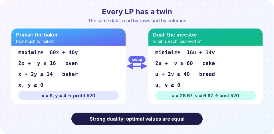
Imagine an investor who wants to buy all of Sunrise Bakery's resources. She offers u dollars per oven hour and v dollars per baker hour. The owner will sell only if the offer is at least as good as using the resources to bake. A cake batch uses 2 oven hours and 1 baker hour and earns $60, so the offer for those resources must be at least 60: 2u + v ≥ 60. Likewise for bread: u + 2v ≥ 40. The investor wants to pay as little as possible for the 16 oven hours and 14 baker hours:
Primal (the baker)                  Dual (the investor)
maximize   60x + 40y                minimize   16u + 14v
subject to 2x +  y ≤ 16   (oven)   subject to 2u +  v ≥ 60   (cake)
            x + 2y ≤ 14   (baker)               u + 2v ≥ 40   (bread)
            x, y ≥ 0                            u, v ≥ 0
Compare the two problems: the profits (60, 40) of the primal became the right-hand sides of the dual, the right-hand sides (16, 14) became the dual's objective coefficients, and the constraint matrix was transposed (rows became columns). A ≤ constraint in a maximization corresponds to a ≥ constraint in the dual. In general, the dual of "maximize c·x subject to Ax ≤ b, x ≥ 0" is "minimize b·y subject to Aᵀy ≥ c, y ≥ 0".
Weak and strong duality
Weak duality. For any feasible primal plan and any feasible dual prices, the profit is at most the price paid: 60x + 40y ≤ 16u + 14v. The investor's offer is always an upper bound on what the baker can earn. (Why? The offer of at least 60 for cake resources covers the cake profit, and so on, summed over the plan.)
Strong duality. If both problems have optimal solutions, their optimal values are equal. Here both are $520. The investor's smallest acceptable offer equals the baker's best profit, so there is no gain from trade.
This is a powerful certificate. If you find a feasible plan with profit 520 and feasible prices with total 520, then both are optimal, and nobody needs to trust the solver.
Press Run (or Ctrl + Enter) to see the result here.
Program input · what you'd type while the program runs
Type the answers before you press Run, one per line. Each time the program reads a line (with input()), it gets the next line from this box.
The dual solution is u = 80/3 ≈ 26.67 dollars per oven hour and v = 20/3 ≈ 6.67 dollars per baker hour, exactly the numbers you found in the simplex tableau. Check: 16 · 80/3 + 14 · 20/3 = 1560/3 = 520.
Complementary slackness
Optimal primal and dual solutions fit together in a precise way.
- If a resource has slack, its price is zero. If the baker does not use all the oven hours, one more oven hour is worth nothing.
- If a resource has a positive price, it is fully used. Only a scarce resource has value.
- If a product is made, its dual constraint holds with equality: the resources it uses are valued exactly at its profit, so it breaks even in resource terms.
- If a product's resources are worth more than its profit, the product is not made.
The last rule explains why the Oak Lane Workshop of Chapter 2 made no shelves. With prices of 0 for wood, 5 for labor and 30 for finishing, a shelf (4 wood, 3 labor hours, 2 finishing hours) uses resources worth 4·0 + 3·5 + 2·30 = 75, more than its profit of 60. The difference, 75 − 60 = 15, is the reduced cost of shelves: the profit per shelf would have to rise by $15 before shelves enter the plan.
Sensitivity: how robust is the answer?
Data are never exact, so we ask how far a number may move before the answer changes. There are two kinds of question.
Right-hand-side ranging
For the oven, the shadow price 26.67 is valid only while the same two constraints stay binding. Keep the baker at 14 hours and let the oven hours be b₁. Solving 2x + y = b₁ and x + 2y = 14 gives x = (2b₁ − 14)/3 and y = (28 − b₁)/3. Both must be nonnegative, so 7 ≤ b₁ ≤ 28. Inside this range, each extra oven hour adds $26.67. Outside it, the baker constraint or the sign limits take over and the price changes: with more than 28 oven hours the baker's hours limit the plan (at most x = 14 cakes), and the extra oven hours are worthless.
Similarly the baker's hours b₂ may range over 8 ≤ b₂ ≤ 32 with the shadow price 6.67 valid.
Objective-coefficient ranging
The plan (6, 4) is optimal as long as the iso-profit line's slope lies between the slopes of the two binding constraints. With bread profit fixed at $40, the cake profit c₁ may vary between $20 and $80 without changing the plan. Check the endpoints: at c₁ = 80, the plan (8, 0) earns 640 and (6, 4) earns 480 + 160 = 640, a tie; above 80 cakes alone are better. At c₁ = 20, (6, 4) earns 120 + 160 = 280, a tie with (0, 7) earning 280.
Press Run (or Ctrl + Enter) to see the result here.
Program input · what you'd type while the program runs
Type the answers before you press Run, one per line. Each time the program reads a line (with input()), it gets the next line from this box.
Press Run (or Ctrl + Enter) to see the result here.
Program input · what you'd type while the program runs
Type the answers before you press Run, one per line. Each time the program reads a line (with input()), it gets the next line from this box.
Read the table: the plan stays at (6, 4) for cake profits from 20 to 80 and jumps to a different corner outside that range, as predicted. (At the endpoints the solver may return either tied corner.)
Using sensitivity in practice
A typical sensitivity report from a solver lists, for each variable, its value, reduced cost and the allowable range of its objective coefficient, and for each constraint, its slack, shadow price and the allowable range of the right-hand side. Managers can use it directly:
- Where to invest. Resources with high shadow prices are worth expanding, up to the end of their range.
- Where not to invest. Resources with slack have price zero.
- Which numbers to measure carefully. Parameters that sit near the edge of their allowable range deserve better data.
- Which products to reprice. A product's reduced cost says how much its price should rise (or its resource use fall) before it becomes attractive.
Common misconceptions
"A shadow price is the market price of the resource." It is the model's value of one extra unit, valid within a range. Compare it with the market price to decide whether to buy.
"If a resource has price zero, it is unimportant." It is unimportant at the margin; removing a lot of it would make it binding.
"Sensitivity analysis changes the model." It does not: it reports how far the numbers can move with the same optimal basis.
Check your understanding
Quick check · 5 questions
of 5 answered You scored / 5 · perfect!
-
1. In the dual of the bakery model, what do the variables u and v represent?
Dual variables price the resources of the primal constraints. -
2. What does strong duality say?
If both problems have optimal solutions, their optimal values are the same. -
3. A resource has slack at the optimum. By complementary slackness, its shadow price is...
An unused resource has no value at the margin. -
4. The oven shadow price of 26.67 is valid for oven hours between 7 and 28. What happens to the value of an extra hour beyond 28?
Outside the range the set of binding constraints changes, so the value changes. -
5. With bread profit at $40, for what cake profits does (6, 4) stay optimal?
The optimal basis remains optimal while the objective slope lies between the slopes of the two binding constraints.
Summary
- The dual prices the primal's resources; its variables are the shadow prices.
- Weak duality bounds the primal by any dual-feasible price; strong duality makes the optimal values equal (520 for the bakery).
- Complementary slackness: slack means zero price; positive price means the resource is fully used; products that are made break even.
- Reduced cost tells how much a product's profit must rise to enter the plan.
- Sensitivity ranges show where shadow prices and the optimal plan remain valid.
Track your progress
Create a free account to tick off lessons and pick up where you left off on any device.
of Operations Research lessons completed