


















Lesson 38 of 49 · Decision Analysis and Game Theory
Chapter 7 Review: Decision Analysis and Game Theory
Review chapter 7 with a one-page picture, a recap table, a reusable decision-tree roll-back function and a ten-question quiz on EMV, EVPI and zero-sum games.
You now have a toolkit for choices made without full knowledge. Against chance you can score alternatives with attitude-based criteria or with expected value, draw a decision tree and roll it back, and calculate what information is worth. Against a rival you can look for a saddle point, strip away dominated strategies and compute mixed strategies, by formula for 2 x 2 games and by linear programming for larger ones.
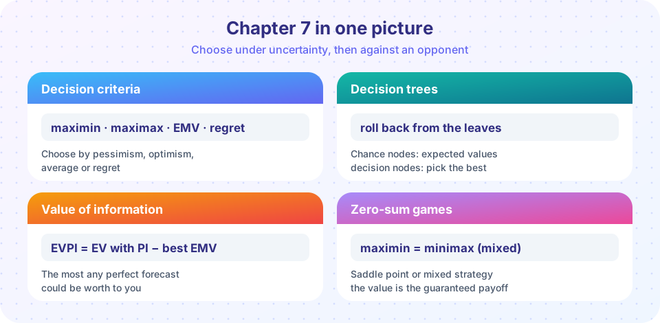
What you will learn
- To recall which tool fits which kind of uncertain decision.
- To recompute any tree with a short program.
- To check your understanding of the chapter's formulas.
The recap table
| Tool | Use it when | Key rule |
|---|---|---|
| Maximin / maximax / Hurwicz / Laplace | No probabilities, a stated attitude | Score each option, pick the best score |
| Minimax regret | You fear missing the best option | Pick the smallest worst regret |
| EMV and decision tree | Probabilities are available | Chance node: average; decision node: best |
| EVPI | Deciding whether to buy a forecast | EV with perfect information − best EMV |
| Bayes' rule and EVSI | A study or test is imperfect | Update probabilities, 0 ≤ EVSI ≤ EVPI |
| Saddle point | Zero-sum game, pure strategies | maximin = minimax |
| 2 x 2 mixed strategy | No saddle point | p = (d − c)/(a + d − b − c), v = (ad − bc)/(a + d − b − c) |
| LP for matrix games | Larger games | Maximize v with Σ x_i A[i][j] ≥ v for each column |
A reusable roll-back function
Decision trees can be coded as nested data. A decision node holds named options, a chance node holds (probability, subtree) pairs, and a leaf is just a number. One recursive function rolls the whole tree back.
Press Run (or Ctrl + Enter) to see the result here.
Program input · what you'd type while the program runs
Type the answers before you press Run, one per line. Each time the program reads a line (with input()), it gets the next line from this box.
The second tree reuses the posterior expected values from the previous lesson. The survey brings the expected profit to about 67.3, so paying 2 leaves about 65.3, which is above 64 and therefore worth buying, while a price of 5 would not be.
Two mixed worked problems
Problem A. A firm chooses between project A (60 percent chance of +50, 40 percent chance of −20) and project B (a sure +15).
EMV(A) = 0.6 × 50 + 0.4 × (−20) = 22,EMV(B) = 15, so EMV favors A.- Maximin compares the worst cases: −20 for A, +15 for B, so maximin picks B. A risk-averse firm that cannot survive a −20 loss would choose B even though its EMV is lower.
- EVPI: with perfect information you would take A in the strong-market state (50) and B in the weak state (15), for
0.6 × 50 + 0.4 × 15 = 36. SoEVPI = 36 − 22 = 14; no forecast is worth more than 14.
Problem B. In matching pennies the row player wins 1 if the coins match and loses 1 otherwise: [[1, −1], [−1, 1]]. There is no saddle point (maximin −1, minimax +1). By the formula, p = (1 + 1)/(1 + 1 + 1 + 1) = 0.5 and v = (1 − 1)/4 = 0. The optimal strategy is to play each side half of the time, and the fair value of the game is 0.
The lesson of problem A is that the "best" option depends on the criterion, and a good analysis shows several: EMV, the worst case and what information would be worth.
Study tips
Draw the tree or the matrix before computing. Most mistakes come from a mislabeled branch, a probability that does not add up to 1, or confusing the row player's payoffs with the column player's losses. After solving a game, test the answer: against each pure column the expected payoff of the row mix should be the same (for a 2 x 2 game without a saddle point).
Common misconceptions
"A mixed strategy is a guess." It is a calculated set of probabilities that equalize the opponent's outcomes.
"Zero-sum means nobody benefits." It means total gains and losses cancel. Many real conflicts are not zero-sum, and cooperation can create value (see Nash equilibria in the game theory track).
Check your understanding
Quick check · 10 questions
of 10 answered You scored / 10 · perfect!
-
1. Option A pays 5, 9, 2 and option B pays 4, 6, 7 in three states. Which one does maximin choose?
The worst cases are 2 for A and 4 for B, so maximin picks B. -
2. An option pays 50 with probability 0.2 and 10 with probability 0.8. What is its EMV?
0.2 × 50 + 0.8 × 10 = 10 + 8 = 18. -
3. Perfect information would give an expected payoff of 60 and the best EMV now is 45. What is the EVPI?
EVPI = 60 − 45 = 15. -
4. Option X pays 20 and 10 in two states; option Y pays 15 and 30. Which option has the smaller maximum regret?
Best payoffs per state are 20 and 30. X's regrets are 0 and 20; Y's are 5 and 0. The maximum regrets are 20 and 5. -
5. Hurwicz with α = 0.6 for an option with best payoff 100 and worst payoff 20 gives what score?
0.6 × 100 + 0.4 × 20 = 60 + 8 = 68. -
6. What is the value of the game with matrix [[1, 3], [4, 5]]?
Row minima are 1 and 4, so maximin = 4; column maxima are 4 and 5, so minimax = 4. The saddle point is 4. -
7. What is the value of the game [[1, 0], [0, 1]]?
a = d = 1 and b = c = 0, so v = (1 − 0)/(1 + 1 − 0 − 0) = 0.5. -
8. Which statement about EVSI and EVPI is true?
An imperfect signal cannot be worth more than perfect knowledge. -
9. P(A) = 0.4, P(+ | A) = 0.9 and P(+ | not A) = 0.2. What is P(A | +)?
P(+) = 0.4 × 0.9 + 0.6 × 0.2 = 0.48, so P(A | +) = 0.36/0.48 = 0.75. -
10. Why does the optimal mixed strategy leave the opponent indifferent between columns?
If one column were better for the opponent, the opponent would use it; equalizing removes any such advantage.
Summary
- Choose a criterion for decisions without probabilities, and EMV with a tree when probabilities exist.
- EVPI caps the value of any information; EVSI values an imperfect study using Bayes' rule.
- Zero-sum games have a value; check for a saddle point, remove dominated strategies and mix when needed.
- Always test the sensitivity of the recommendation to the numbers.
Track your progress
Create a free account to tick off lessons and pick up where you left off on any device.
of Operations Research lessons completed