


















Lesson 28 of 49 · Inventory and Scheduling
Scheduling: Dispatch Rules and Johnson's Rule
Sequence jobs on one machine with SPT and EDD, measure flow time and lateness, and minimize makespan on two machines with Johnson's rule, with code.
A printing shop has four orders waiting. A hospital has five patients needing the same scanner. A cloud server has a queue of batch jobs. In each case the work must be put in some order, and the order changes the outcome even though the total work is exactly the same. Scheduling is the part of operations research that picks the order.
Surprisingly, some scheduling problems have beautifully simple rules that are provably best. Others are among the hardest problems in computer science. This lesson studies the simple ones on a single machine and then a classic two-machine result due to S. M. Johnson (1954).
What you will learn
- The standard measures of schedule quality: completion time, flow time, lateness, tardiness and makespan.
- Why SPT minimizes average flow time and EDD minimizes maximum lateness.
- How to apply Johnson's rule to a two-machine flow shop and compute the makespan.
- Why most larger scheduling problems need heuristics (the topic of chapter 8).
Key terms
Processing time (p): how long a job needs on a machine.
Completion time (C): the clock time when the job finishes; flow time is completion minus release (here, release is time 0, so they coincide).
Due date (d) and lateness (L): L = C − d. It is negative if the job is early; tardiness is max(0, L).
Makespan: the time at which the last job finishes.
Flow shop: every job visits the machines in the same order (machine 1, then machine 2).
One machine, four jobs
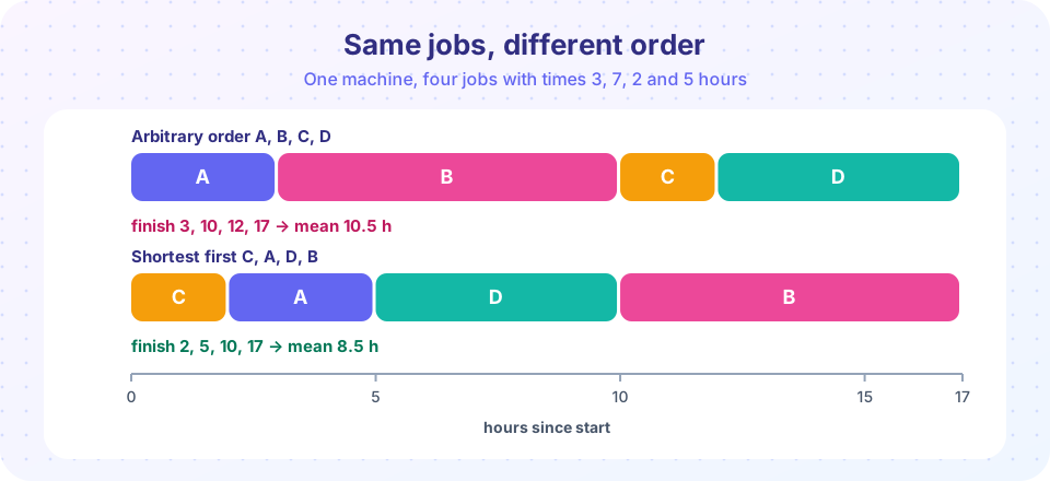
Four jobs wait at time 0 for one machine. Processing times and due dates (hours) are:
| Job | Time p | Due d |
|---|---|---|
| A | 3 | 5 |
| B | 7 | 9 |
| C | 2 | 11 |
| D | 5 | 7 |
The machine can handle one job at a time and never idles. How should we order them? That depends on the objective. With four jobs there are only 4! = 24 sequences, but with 20 jobs there are about 2.4 × 10¹⁸. We need rules.
SPT: shortest processing time first
SPT sorts jobs by p ascending: C, A, D, B. Completion times are 2, 5, 10, 17 and the average is (2 + 5 + 10 + 17) / 4 = 8.5 hours.
Why is this the best average? Use an exchange argument. Suppose two neighbors are in the order (long, short). If you swap them, the short job finishes earlier by the length of the long one, while the long job finishes later by only the length of the short one. The sum of the two completion times drops. Repeating the swap until no pair is out of order leads to SPT, and every swap improved or kept the total. Therefore SPT minimizes the average completion time (and average number of jobs waiting).
EDD: earliest due date first
EDD sorts by d ascending: A (5), D (7), B (9), C (11). Completions are 3, 8, 15, 17 and the lateness values are −2, +1, +6, +6. The maximum lateness is 6 hours. Under SPT the lateness values are C: −9, A: 0, D: +3, B: +8, so the maximum is 8. An exchange argument again proves that EDD minimizes the maximum lateness.
Notice that no rule wins everything:
| Measure | SPT order C, A, D, B | EDD order A, D, B, C |
|---|---|---|
| Average completion time | 8.5 | 10.75 |
| Maximum lateness | 8 | 6 |
| Number of late jobs | 2 | 3 |
Try it
Compare the rules, and verify them against every possible sequence.
Press Run (or Ctrl + Enter) to see the result here.
Program input · what you'd type while the program runs
Type the answers before you press Run, one per line. Each time the program reads a line (with input()), it gets the next line from this box.
The brute-force line confirms the theory: nothing beats SPT's mean completion time or EDD's maximum lateness. The fewest late jobs (2 here, which SPT happens to reach) is a different objective. In general it needs another algorithm, due to Moore and Hodgson, which removes the longest job whenever a job would be late.
Two machines in a row: Johnson's rule
Many shops are flow shops: every job goes through machine 1 (say, cutting) and then machine 2 (say, painting). Machine 2 cannot start a job until machine 1 has finished it, and each machine does one job at a time. We want the shortest makespan.
Here are five jobs with times on each machine:
| Job | Machine 1 | Machine 2 |
|---|---|---|
| J1 | 3 | 6 |
| J2 | 5 | 2 |
| J3 | 1 | 2 |
| J4 | 6 | 6 |
| J5 | 7 | 5 |
Johnson's rule gives an optimal order in two steps:
- Put every job with
time on M1 ≤ time on M2in a first group, sorted by M1 time ascending. - Put every other job in a second group, sorted by M2 time descending.
- The sequence is the first group followed by the second.
For our data the first group is J3 (1, 2), J1 (3, 6), J4 (6, 6), and the second group is J5 (M2 = 5) then J2 (M2 = 2). The order is J3, J1, J4, J5, J2. The idea is simple: send jobs that are quick on machine 1 first, so machine 2 starts working early, and keep jobs that are quick on machine 2 for the end, so machine 2 finishes soon after machine 1 stops.
Press Run (or Ctrl + Enter) to see the result here.
Program input · what you'd type while the program runs
Type the answers before you press Run, one per line. Each time the program reads a line (with input()), it gets the next line from this box.
Johnson's rule is optimal for two machines. With three or more machines the problem becomes NP-hard in general (no known fast exact method), and real shops combine dispatch rules, integer programming (see linear programming) and heuristics such as those in chapter 8.
Beyond these rules
Real schedules also have release times, setup times that depend on the previous job, machines that break, and workers with shifts. Planners often use priority dispatch rules (SPT, EDD, slack time, critical ratio) as fast, transparent defaults, then improve the result with search. The theory here tells you what each rule is good at, so you can choose the one that matches the business goal: speed, punctuality or utilization.
Dispatch rules in practice
In real shops, jobs arrive over time and a planner cannot see the future, so the work is organized by dispatch rules: whenever a machine becomes free, pick the next job by a priority rule. Besides SPT and EDD, popular rules include slack time (due date minus the remaining work minus the current time; the smallest slack goes first), the critical ratio (time left until the due date divided by the remaining processing time; a ratio below 1 means the job is already behind) and first come, first served, which is simple and perceived as fair but ignores both length and urgency.
Which rule is best depends on the goal. A hospital laboratory that wants a low average turnaround time uses something close to SPT. An express courier that has promised delivery times uses due-date-driven rules. A factory with expensive machines may care most about the makespan. Simulation (chapter 6) lets a planner try the rules on a model of the shop before changing the real procedure. In all cases, rules should be paired with a safeguard against starvation: a very long job should not wait forever just because shorter jobs keep arriving.
Reading a Gantt chart
A Gantt chart, like the ones in this lesson, shows time on the horizontal axis and one row per machine. Each bar is a job; the right end of a bar is the completion time. To read the mean completion time, note the right ends of all bars and average them. To find idle time on a machine, look for gaps between bars. In a two-machine chart, check that no bar on machine 2 starts before the same job has finished on machine 1: that is the flow-shop rule, and Johnson's order is designed to make the gaps on machine 2 as small as possible.
Common misconceptions
"There is one best schedule." Best depends on the objective. SPT, EDD and Johnson's rule optimize different measures and can disagree.
"SPT is unfair." It can starve long jobs when short jobs keep arriving. Aging (raising a job's priority as it waits) is a practical fix.
"Johnson's rule works for any number of machines." It is proved only for two machines (and for special three-machine cases).
Check your understanding
Quick check · 5 questions
of 5 answered You scored / 5 · perfect!
-
1. Which rule minimizes the average completion time on one machine?
An exchange argument shows swapping a long job ahead of a short one only increases the total completion time, so SPT is optimal. -
2. Jobs have times 4, 1 and 3. Under SPT, what are the completion times?
SPT order is 1, 3, 4, so completion times are 1, 1 + 3 = 4 and 4 + 4 = 8. -
3. Which rule minimizes the maximum lateness on one machine?
Sequencing by due date prevents any job from being pushed far past its due date and is proved optimal for maximum lateness. -
4. A job takes 3 hours on machine 1 and 8 on machine 2. In which Johnson group is it?
Its M1 time is at most its M2 time, so it belongs to the first group. -
5. What is the makespan?
Makespan is the time at which all jobs are complete.
Summary
- Schedule quality is measured by completion time, lateness, tardiness and makespan; the best order depends on the measure.
- SPT minimizes average completion time and EDD minimizes maximum lateness, both by exchange arguments.
- Johnson's rule orders a two-machine flow shop optimally: short-on-M1 jobs first (ascending), then the rest by descending M2 time.
- Larger shop problems are hard, so planners use rules plus heuristics.
Next: Chapter 5 review
Track your progress
Create a free account to tick off lessons and pick up where you left off on any device.
of Operations Research lessons completed