


















Lesson 30 of 49 · Queueing and Simulation
Chapter 6 Overview: Queueing and Simulation
A map of chapter 6: why lines form, the vocabulary of queueing systems, and how formulas and simulation work together to predict waiting times.
You have waited in a line today, whether at a checkout, in a call-waiting loop or behind a loading bar. Lines are not a sign that someone failed; they are a mathematical consequence of randomness. Even when a bank can serve more customers per hour than arrive, a few customers will show up together, and the line will build up for a while. Queueing theory predicts how long and how often, and simulation lets you answer the questions that formulas cannot.
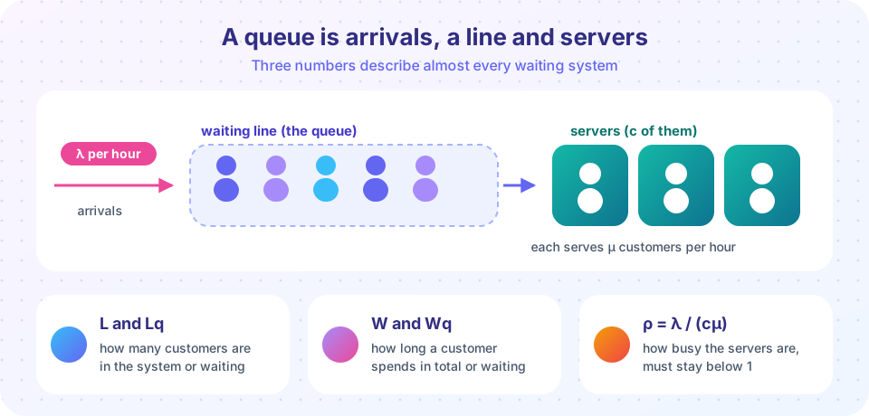
What you will learn
- The vocabulary of a queueing system: arrival rate, service rate, servers, utilization and discipline.
- Why a system that is on average fast enough still has waiting lines.
- How the chapter's three tools (M/M/1, Erlang C, simulation) fit together.
- What to try first and in what order to read the lessons.
Key terms
Arrival rate (λ): average number of customers arriving per unit time.
Service rate (μ): average number a single busy server completes per unit time; the mean service time is 1/μ.
Utilization (ρ): the fraction of time servers are busy, ρ = λ / (cμ) for c servers.
Queue discipline: the rule for who is served next (first come first served, priority, and so on).
Steady state: the long-run behavior after the system has settled, which formulas describe.
Why lines form even with spare capacity
Suppose a clinic's one doctor can see 6 patients an hour, and on average 5 patients arrive per hour. Capacity is bigger than demand, yet patients wait. Why? Because arrivals come randomly. Sometimes three patients arrive within ten minutes, and the doctor, who can see only one at a time, builds a backlog that takes a while to clear. When the doctor is idle, that idle time cannot be saved for later. This asymmetry (unused capacity vanishes, but backlog persists) is the heart of every waiting line.
The consequence is a law you will see numerically in the next lessons: the closer utilization gets to 100 percent, the more dramatically waiting times grow. A system that is 95 percent busy has not "5 percent spare"; it has long lines.
The big picture
Describe the system
Measure it
Predict it
Formulas for steady state
Test it
Any rule, any data
A first look
Before any formulas, simulate a one-server queue and see how the average wait reacts to the arrival rate. The code uses a classic recursion: a customer's wait equals the previous customer's wait plus the previous service time minus the gap between arrivals, but never below zero.
Press Run (or Ctrl + Enter) to see the result here.
Program input · what you'd type while the program runs
Type the answers before you press Run, one per line. Each time the program reads a line (with input()), it gets the next line from this box.
Notice how the waits change slowly at first and then jump. Lesson 2 gives the exact formula for this curve.
Where the chapter goes
| Lesson | What you will learn |
|---|---|
| The M/M/1 queue | Exact formulas for one server, Little's law and the explosive effect of high utilization |
| Several servers: Erlang C | Staffing a call center or checkout bank, and the benefit of pooling |
| Discrete-event simulation | Building a simulator, running replications, warm-up and confidence intervals |
| Chapter 6 review | A one-page recap and a ten-question quiz |
If this chapter makes you curious, the full queueing theory track goes much further, and Monte Carlo simulation studies the random-number side in depth.
Common misconceptions
"If capacity exceeds demand, there is no line." Random bunching creates lines even when the average capacity is larger than the average demand.
"Waiting grows linearly with utilization." It grows like 1/(1 − ρ), so it rises slowly and then steeply.
"Simulation is the same as guessing." A simulation follows exact rules; its randomness is controlled and its uncertainty can be measured.
Check your understanding
Quick check · 4 questions
of 4 answered You scored / 4 · perfect!
-
1. A server completes 8 customers per hour when busy. What is the mean service time?
The mean service time is 1/μ = 1/8 hour = 7.5 minutes. -
2. Customers arrive at 12 per hour and one server handles 15 per hour. What is the utilization?
ρ = λ/μ = 12/15 = 0.8. -
3. Why do lines form when average capacity exceeds average demand?
Bunched arrivals create backlogs, while idle time in quiet periods is lost. -
4. As utilization approaches 1, the average wait...
Waiting time scales like 1/(1 − ρ), which explodes as ρ nears 1.
Summary
- Queueing models describe arrivals, service and servers; key measures are
L,Lq,W,Wqandρ. - Randomness creates lines even when capacity exceeds demand.
- Waiting time rises steeply as utilization approaches 100 percent.
- Formulas (M/M/1, Erlang C) give fast answers; simulation handles everything else.
Next: The M/M/1 queue
Track your progress
Create a free account to tick off lessons and pick up where you left off on any device.
of Operations Research lessons completed