


















Lesson 13 of 49 · Linear and Integer Programming
The Graphical Method for Linear Programs
Solve two-variable linear programs by drawing the feasible region, finding corner points and sliding the profit line, including infeasible and unbounded cases.
With only two decision variables, a linear program can be solved with a ruler and a pencil. You draw each constraint as a line, shade the plans that obey all of them, and look for the best point. The method does not scale beyond two variables, but it shows why linear programming works, and every idea in it carries over to the simplex method of the next lesson. In this lesson you solve the Sunrise Bakery problem completely by picture, then explore the three special cases that can occur.
What you will learn
- How to draw a constraint and shade the feasible side.
- How to find corner points by solving two equations.
- How to use an iso-profit line to find the optimum.
- What infeasible, unbounded and multiple-optimum problems look like.
Key terms
Half-plane: all points on one side of a line, such as 2x + y ≤ 16.
Feasible region: the overlap of all the half-planes.
Corner point: a vertex of the feasible region where two boundary lines cross.
Iso-profit line: all plans that give the same profit; for 60x + 40y these are parallel lines.
Alternative optima: several plans that all achieve the best objective value.
Step 1: draw the constraints
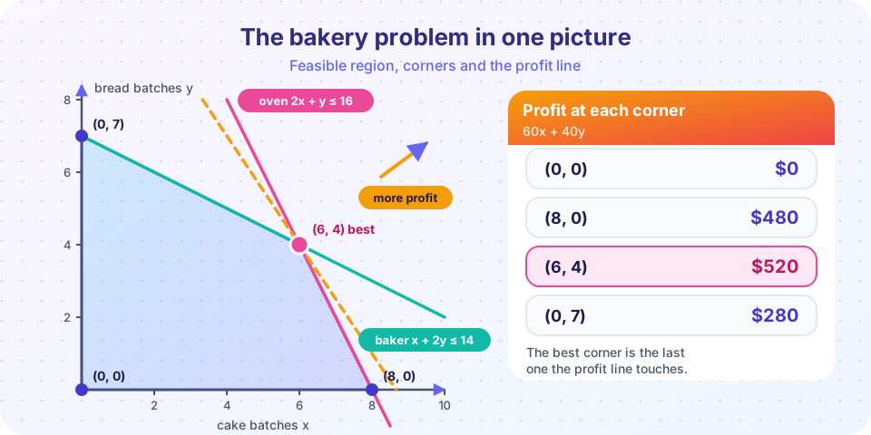
The model is: maximize 60x + 40y subject to 2x + y ≤ 16, x + 2y ≤ 14, x ≥ 0, y ≥ 0.
To draw 2x + y ≤ 16, first draw the boundary 2x + y = 16. Find two points on it by setting one variable to zero: x = 0 gives y = 16, and y = 0 gives x = 8. Join them. Then decide which side to shade by testing a point that is not on the line, the origin: 2·0 + 0 = 0 ≤ 16 is true, so the side with the origin is feasible.
For x + 2y ≤ 14: the intercepts are (14, 0) and (0, 7), and the origin satisfies it, so again the origin's side is feasible.
The constraints x ≥ 0 and y ≥ 0 keep us in the first quadrant. The feasible region is where all four shaded areas overlap.
Step 2: find the corner points
The region in the picture is a four-sided polygon. Its corners are:
| Corner | How you get it | Coordinates |
|---|---|---|
| Origin | x = 0 and y = 0 |
(0, 0) |
| On the x-axis | y = 0 with 2x + y = 16 |
(8, 0) |
| Where the two limits cross | solve 2x + y = 16 and x + 2y = 14 |
(6, 4) |
| On the y-axis | x = 0 with x + 2y = 14 |
(0, 7) |
To find the third corner, subtract: multiply the first equation by 2 to get 4x + 2y = 32, subtract x + 2y = 14 to get 3x = 18, so x = 6, and then y = 16 − 12 = 4.
Note that the points (14, 0) and (0, 16) where the lines meet the axes are not corners of the region: they violate the other constraint.
Step 3: compare the corners, or slide the profit line
Evaluate the objective at each corner:
| Corner | Profit 60x + 40y |
|---|---|
| (0, 0) | 0 |
| (8, 0) | 480 |
| (6, 4) | 520 |
| (0, 7) | 280 |
The largest is $520 at (6, 4).
There is a second way to see it. All plans with profit P lie on the line 60x + 40y = P. For different values of P these are parallel lines, and a larger P means a line further from the origin. Start with a small profit and slide the line away from the origin, in the direction (60, 40). The last point of the region the line touches is the optimum. Since the region is a polygon, the last contact is a corner. That is the central fact of linear programming.
Press Run (or Ctrl + Enter) to see the result here.
Program input · what you'd type while the program runs
Type the answers before you press Run, one per line. Each time the program reads a line (with input()), it gets the next line from this box.
Reading the picture: binding constraints and shadow prices
At (6, 4) both the oven and the baker constraints hold with equality: they are binding, as you saw in Chapter 2. If you add oven hours, the oven line moves outward, the corner slides along the baker line, and the profit grows. The rate of growth is the oven's shadow price (the duality lesson computes it as $26.67 per hour). Pictures like this explain shadow prices better than any formula.
Special cases
Not every LP has one neat answer. Three other outcomes can occur.
Infeasible. The constraints contradict each other, so the feasible region is empty. Add the rule x + y ≥ 12 to the bakery. No plan can satisfy it together with the oven and baker limits (the largest possible x + y is 10), so no feasible plan exists. A solver reports status "infeasible". In practice this signals a data error or an impossible demand.
Unbounded. The region stretches to infinity in the direction in which the objective improves, so the objective can grow without limit. For example, maximize x + y subject only to x − y ≤ 2 and x, y ≥ 0. Real businesses cannot make infinite profit, so an unbounded model means a missing constraint.
Multiple optima. If the iso-profit line is parallel to a boundary edge, then an entire edge is optimal. Change the profits to $60 for cakes and $30 for bread. The objective 60x + 30y is parallel to the oven line 2x + y = 16, so every plan on the segment from (8, 0) to (6, 4) earns $480. The solver returns one corner, but you can choose any plan along the edge, for example the one that is easiest to run.
Press Run (or Ctrl + Enter) to see the result here.
Program input · what you'd type while the program runs
Type the answers before you press Run, one per line. Each time the program reads a line (with input()), it gets the next line from this box.
The point (7, 2) lies on the oven line between the two corners (2·7 + 2 = 16) and is feasible for the baker (7 + 4 = 11 ≤ 14), so it also earns $480.
Graphical minimization
Minimization works the same way, except that you slide the cost line towards the origin and stop at the last feasible contact. Consider: minimize 3x + 2y subject to x + y ≥ 4, x + 3y ≥ 6 and x, y ≥ 0. The feasible region lies above and to the right of both lines and is unbounded, but the cost still has a finite minimum because costs cannot go below zero. The corners are (0, 4), (3, 1) (solve the two equations) and (6, 0). Their costs are 8, 11 and 18, so the cheapest plan is (0, 4) with cost 8.
Why this does not scale (and why it still matters)
With three variables the constraints become planes and the region a solid; you can still sketch it. With ten variables you cannot draw anything, and the number of corners can be huge: a region defined by m constraints in n variables can have up to m choose n corners. The simplex method (next lesson) walks along the edges of the region from corner to corner without visiting them all, but the geometric picture you built here is exactly what it is doing.
Common misconceptions
"The best point is where all the lines cross." Only constraints that bind at the optimum pass through it; others may be far away.
"If the solver returns a corner, there is only one best plan." With alternative optima, other plans are equally good; the solver simply picks one.
"An unbounded result means a very good business." It means the model forgot a limit.
Check your understanding
Quick check · 5 questions
of 5 answered You scored / 5 · perfect!
-
1. How do you decide which side of the line 2x + y = 16 to shade for 2x + y ≤ 16?
Substitute a test point: the origin gives 0 ≤ 16, which is true, so that side is feasible. -
2. What are the coordinates where 2x + y = 16 and x + 2y = 14 cross?
From 2x + y = 16 and x + 2y = 14 you get x = 6 and y = 4. -
3. What does an unbounded LP indicate?
An unbounded region in the improving direction usually signals a missing constraint. -
4. When do alternative optima occur?
If the iso-profit line lies along a boundary edge, every point of that edge is optimal. -
5. For the model max 60x + 40y, what is the profit at the corner (0, 7)?
60·0 + 40·7 = 280.
Summary
- Draw each constraint, shade the feasible side by testing a point, and intersect the shaded areas.
- The best plan is at a corner; compute corners by solving two boundary equations and compare the objective.
- Iso-profit lines are parallel; slide them until the last contact with the region.
- Infeasible, unbounded and multiple-optima outcomes each have a clear geometric meaning.
- The method generalizes to the simplex method.
Next: The Simplex Method
Track your progress
Create a free account to tick off lessons and pick up where you left off on any device.
of Operations Research lessons completed