


















Lesson 34 of 49 · Queueing and Simulation
Chapter 6 Review: Queueing and Simulation
Review chapter 6 with a one-page picture, a formula table, a checker for Little's law and a ten-question quiz on M/M/1, Erlang C and simulation.
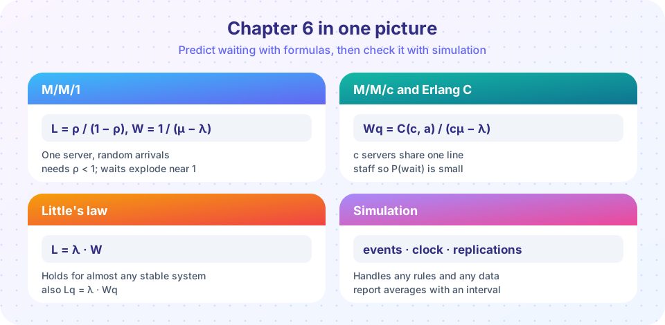
This chapter showed that waiting is a mathematical object. You met the M/M/1 queue and its steep climb near full utilization, the Erlang C model for several servers and the benefits of pooling, and discrete-event simulation for everything else. This review lines the pieces up and gives you a ten-question check.
What you will learn
- To pick between a formula and a simulation for a waiting-line problem.
- To recall the key formulas and the conditions they need.
- To check results for consistency with Little's law.
The recap table
| Topic | Key facts |
|---|---|
| Notation | λ arrivals per time, μ services per time per server, ρ = λ/(cμ), stable only if ρ < 1 |
| M/M/1 | p_n = (1 − ρ)ρⁿ, L = ρ/(1 − ρ), Lq = ρ²/(1 − ρ), W = 1/(μ − λ), Wq = ρ/(μ − λ) |
| Little's law | L = λW and Lq = λWq, for almost any stable system |
| Erlang C | C(c, a) is the chance of waiting; Wq = C/(cμ − λ); P(Wq > t) = C·e^{−(cμ − λ)t} |
| Pooling | One shared line beats separate lines, especially at high load |
| Simulation | State, event list, clock; validate, discard warm-up, replicate, report intervals |
| Variability | At the same utilization, more variable service means longer waits |
Consistency check
Little's law is a free test. If your formula for L and your formula for W do not satisfy L = λW, something is wrong. The code below checks it for several M/M/c systems.
Press Run (or Ctrl + Enter) to see the result here.
Program input · what you'd type while the program runs
Type the answers before you press Run, one per line. Each time the program reads a line (with input()), it gets the next line from this box.
The last column is zero (up to rounding) in every row, as Little's law promises. The row 30, 10, 4 has an offered load of 3 Erlangs on 4 servers, so it is stable but long-lined, while adding the fifth server in the next row cuts the wait sharply.
Two mixed worked problems
Problem A. Customers arrive at 3 per hour at a counter with one clerk who serves 4 per hour. Compute the average time in the queue. The company considers adding a second clerk (same speed, one shared line). What happens?
- One clerk:
ρ = 0.75,Wq = ρ/(μ − λ) = 0.75/(4 − 3) = 0.75hour = 45 minutes. - Two clerks:
a = 0.75,ρ = 0.375. The sum fork = 0, 1is1 + 0.75 = 1.75; the waiting term is(0.75²/2)/(1 − 0.375) = 0.28125/0.625 = 0.45. SoC = 0.45/(1.75 + 0.45) ≈ 0.205andWq = 0.205/(8 − 3) ≈ 0.041hour, about 2.5 minutes.
A second clerk cuts the wait from 45 to about 2.5 minutes, a drop of more than 90 percent, because the system moves from a heavily loaded to a lightly loaded state. That is the nonlinearity of the first lesson in action.
Problem B. A simulation of the queue gives 10 replications with average waits of 40, 52, 47, 44, 49, 38, 51, 46, 43 and 50 minutes. The mean is 46 minutes and the standard deviation is about 4.7. With t = 2.26 (9 degrees of freedom) the half-width of a 95 percent interval is 2.26 × 4.7/√10 ≈ 3.4, so the interval is about [42.6, 49.4]. Ten replications pin the answer down to within about 3.4 minutes.
Study tips
Practice moving between the three views of a queue: the formula (fast, exact under assumptions), the simulation (flexible, noisy) and the picture (the hockey-stick curve). If you can predict from the picture roughly what the formula will say, you understand the model, not just the algebra.
Common misconceptions
"A formula and a simulation are rivals." They complement each other: use formulas for fast answers and for validating the simulator, and the simulator for anything the formulas cannot express.
"Little's law needs exponential times." It holds for almost any stable system, which is why it is so useful as a check.
Check your understanding
Quick check · 10 questions
of 10 answered You scored / 10 · perfect!
-
1. An M/M/1 queue has λ = 2 per hour and μ = 5 per hour. What is L?
ρ = 0.4 and L = 0.4/0.6 ≈ 0.67. -
2. λ = 9 per hour and μ = 10 per hour in an M/M/1 queue. What is W?
W = 1/(μ − λ) = 1/(10 − 9) = 1 hour. -
3. 30 customers are in a shop on average, and 6 arrive per hour. By Little's law, how long does each stay?
W = L/λ = 30/6 = 5 hours. -
4. Calls arrive at 30 per hour and each agent handles 10 per hour. What is the smallest number of agents for a stable system?
The offered load is exactly 3 Erlangs, and stability needs more than 3 servers, so 4. -
5. Why does pooling servers reduce waiting?
Separate lines can leave one server idle while others have queues; a shared line removes that waste. -
6. C(c, a) = 0.5 and cμ − λ = 10 per hour. What is Wq?
Wq = 0.5/10 = 0.05 hour = 3 minutes. -
7. In an M/M/1 queue with ρ = 0.7, what is the probability of at least 2 customers in the system?
P(n ≥ k) = ρᵏ, so P(n ≥ 2) = 0.7² = 0.49. -
8. Why discard a warm-up period in a simulation?
Starting empty biases early observations, so they are dropped. -
9. At the same utilization, which service pattern gives the longest waits?
Waiting grows with the variability of service times. -
10. 20 replications give a mean of 40 minutes with a standard deviation of 10 and t = 2.09. What is the half-width of a 95% interval?
2.09 × 10 / √20 ≈ 4.67 minutes.
Summary
- M/M/1 and Erlang C give exact steady-state answers under their assumptions; waiting explodes as
ρ → 1. - Little's law
L = λWlinks numbers of customers and times, and doubles as a consistency check. - Pooling servers shortens waits at no cost.
- Simulation handles real-world rules, but needs validation, warm-up removal and replications.
Track your progress
Create a free account to tick off lessons and pick up where you left off on any device.
of Operations Research lessons completed