


















Lesson 37 of 49 · Decision Analysis and Game Theory
Zero-Sum Games: Saddle Points and Mixed Strategies
Solve two-player zero-sum games: find saddle points, remove dominated strategies, compute 2x2 mixed strategies and solve any matrix game with linear programming.
In a decision against nature, the world does not mind what you choose. In a game, the other side does. If you always choose the same action, a clever rival will learn it and exploit it. The question becomes: what strategy gives me the best guaranteed result, whatever the opponent does? For two players whose interests are exactly opposed, the answer is one of the most elegant results in applied mathematics, the minimax theorem, proved by John von Neumann in 1928.
This lesson shows you how to solve such games by hand and by computer.
What you will learn
- How to read a payoff matrix and find a saddle point with maximin and minimax.
- How to remove dominated strategies to simplify a game.
- How to compute the optimal mixed strategy and value of a 2 x 2 game.
- How to solve any matrix game as a linear program.
Key terms
Zero-sum game: whatever one player wins, the other loses, so the payoffs add up to zero.
Pure strategy: always choosing one fixed action. Mixed strategy: choosing actions at random with fixed probabilities.
Saddle point: an entry that is both the smallest in its row and the largest in its column; it is a stable pure-strategy solution.
Value of the game (v): the payoff the row player can guarantee, and the column player can hold the row player to.
Dominated strategy: one that is never better than another and sometimes worse, so it can be dropped.
The payoff matrix
Two players move at the same time. The row player chooses a row, the column player chooses a column, and the entry shows what the column player pays the row player (negative means the row player pays). The row player wants a large entry, the column player a small one.
Here is a game:
| B1 | B2 | |
|---|---|---|
| A1 | 3 | −1 |
| A2 | −2 | 4 |
Think like the row player. If you choose A1, the worst you can get is −1 (if B picks B2). If you choose A2, the worst is −2. The maximin strategy chooses the row with the best worst case: A1, guaranteeing at least −1.
The column player thinks the opposite way. Choosing B1 risks paying 3 (the largest entry in column B1), and B2 risks paying 4. The minimax choice is B1, holding the loss to at most 3.
Since maximin = −1 and minimax = 3 are different, no entry is a saddle point and neither player has a stable pure strategy. If A plays A1, B replies B2 and A regrets not playing A2, and so on. The cycle never ends. The solution is to randomize.
When a saddle point exists
Another game:
| B1 | B2 | B3 | |
|---|---|---|---|
| A1 | 5 | 3 | 6 |
| A2 | 2 | 1 | 8 |
| A3 | 4 | 0 | 3 |
Row minima are 3, 1 and 0, so maximin = 3 (row A1). Column maxima are 5, 3 and 8, so minimax = 3 (column B2). They agree: the entry 3 at (A1, B2) is a saddle point. Neither player gains by switching if the other sticks to it. The value of the game is 3, achieved with pure strategies.
Dominance
Before solving, simplify. If row i is at least as good as row k in every column, then row k is dominated and the row player will never need it. The same holds for columns, with the opposite inequality, because the column player wants small entries. Remove dominated rows and columns repeatedly; the remaining game has the same value.
Example: in the matrix with rows [3, 1], [2, 4] and [0, 0], the last row is dominated by the first (3 > 0 and 1 > 0), so it can be deleted.
Mixed strategies for a 2 x 2 game
For a game with entries a, b in the top row and c, d in the bottom row and no saddle point, let the row player play row 1 with probability p. Against column 1 the expected payoff is p·a + (1 − p)·c, and against column 2 it is p·b + (1 − p)·d. The row player should choose p to equalize the two, so the opponent cannot exploit a preference:
p = (d − c) / (a + d − b − c), q = (d − b) / (a + d − b − c), v = (ad − bc) / (a + d − b − c)
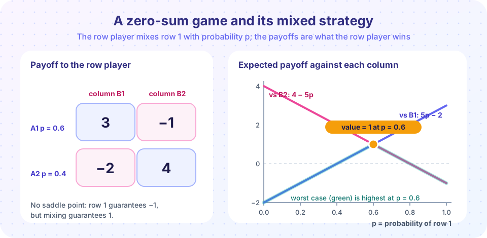
where q is the probability that the column player picks column 1. For our matrix a = 3, b = −1, c = −2, d = 4, the denominator is 3 + 4 + 1 + 2 = 10. Then p = (4 + 2)/10 = 0.6, q = (4 + 1)/10 = 0.5 and v = (12 − 2)/10 = 1. Check: against column 1, 0.6 × 3 + 0.4 × (−2) = 1; against column 2, 0.6 × (−1) + 0.4 × 4 = 1. The game favors the row player by 1 per round, and no counter-strategy can change this.
The figure at the top shows the idea: each column choice defines a line in p. The row player's guaranteed payoff is the lower envelope of the lines, and the best p is where that envelope peaks, at the crossing.
Try it
First, an interactive solver for any 2 x 2 matrix. Edit the four numbers.
Any matrix game as a linear program
For larger games, use linear programming (see the linear programming track). The row player chooses probabilities x_1, ..., x_m and a guaranteed value v to
maximize v subject to Σ_i x_i · A[i][j] ≥ v for every column j, Σ_i x_i = 1, x ≥ 0
The column player's problem is its dual, which is why both players reach the same value. The next TryIt solves several games with SciPy: the 2 x 2 game above, the saddle game, and rock-paper-scissors (win +1, lose −1, tie 0).
Press Run (or Ctrl + Enter) to see the result here.
Program input · what you'd type while the program runs
Type the answers before you press Run, one per line. Each time the program reads a line (with input()), it gets the next line from this box.
The first game returns value 1 with row strategy [0.6, 0.4], matching our hand calculation. The saddle game puts all weight on row A1, and rock-paper-scissors returns the uniform mix 1/3, 1/3, 1/3 with value 0.
You can also test the guarantee by simulation: whatever fixed or random choices the column player makes, the long-run average payoff of the optimal mix never falls below the value.
Press Run (or Ctrl + Enter) to see the result here.
Program input · what you'd type while the program runs
Type the answers before you press Run, one per line. Each time the program reads a line (with input()), it gets the next line from this box.
Every answer is close to 1 because the mix p = 0.6 equalizes the two columns: whatever the column player does, the row player's expected payoff is exactly 1. That is also why the column player is happy to play its own optimal mix q = 0.5: nothing better is available. If the row player strayed from p = 0.6, a column player who notices could push the average below 1.
Why mix at all?
Mixing is not about being unpredictable for its own sake. It is the only way to stop an observant opponent from exploiting you. Football penalty kicks, tennis serve placement and poker bluffing are common illustrations: a player who always goes the same way is easy to beat. Mixed strategies also arise in military and security scheduling, where patrols must not follow a pattern an attacker can learn.
Not every conflict is zero-sum. When both sides can gain, as in negotiations or pricing, the relevant concept is the Nash equilibrium (John Nash, 1950), which the game theory track covers.
Common misconceptions
"A mixed strategy means choosing randomly with equal chances." The probabilities are exactly the ones that make the opponent indifferent. They are rarely 50/50.
"If I know the matrix, I can predict the opponent." Only if the opponent is not playing optimally. Against an optimal opponent, the best you can do is secure the value.
"The value is the payoff in each round." It is the long-run average payoff. A single round can pay −1 or +3.
Check your understanding
Quick check · 5 questions
of 5 answered You scored / 5 · perfect!
-
1. Row minima of a matrix are 2, 5 and 1, and column maxima are 7, 5 and 9. Is there a saddle point?
Maximin = 5 and minimax = 5, so the entry 5 is a saddle point and the value is 5. -
2. In the game [[2, 6], [4, 3]] with no saddle point, what is the value? (Use v = (ad − bc)/(a + d − b − c).)
a = 2, b = 6, c = 4, d = 3: v = (ad − bc)/(a + d − b − c) = (6 − 24)/(2 + 3 − 6 − 4) = (−18)/(−5) = 3.6. -
3. Which description matches a dominated row?
A dominated row is never better than some other row, so the row player can discard it. -
4. Why does the optimal mixed strategy equalize the opponent's expected payoffs?
If the opponent's choices give different results, the opponent would favor the best one; equalizing removes that incentive. -
5. What is the value of rock-paper-scissors?
The game is symmetric, so neither player can guarantee more than 0, and the uniform mix achieves it.
Summary
- In a zero-sum game, maximin (row) and minimax (column) bound the value; if they agree, there is a saddle point.
- Remove dominated rows and columns first.
- For a 2 x 2 game without a saddle point, mix so the opponent's payoffs are equal:
p = (d − c)/(a + d − b − c)andv = (ad − bc)/(a + d − b − c). - Every finite zero-sum game has a value (minimax theorem) that can be found by linear programming.
Next: Chapter 7 review
Track your progress
Create a free account to tick off lessons and pick up where you left off on any device.
of Operations Research lessons completed