


















Lesson 26 of 49 · Inventory and Scheduling
Production Runs and Quantity Discounts
Extend the EOQ model to a factory that makes its own stock (EPQ) and to suppliers that sell cheaper in bulk, with worked examples and code.
The EOQ model assumes an order arrives all at once, like a truck unloading at the dock. Many items do not arrive that way. A bottling plant fills its own warehouse bottle by bottle, and while it is running, customers keep buying. Other times the supplier changes the price if you buy more. Both situations are small variations of the EOQ idea, and both are worth learning because they show how an operations researcher adapts a model instead of discarding it.
What you will learn
- How the EPQ (economic production quantity) model changes the average stock and the optimum.
- How to compute run length, peak stock and yearly cost for a production run.
- How to solve an all-units quantity discount problem step by step.
- Why the cheapest unit price can beat the cheapest holding policy.
Key terms
P: production rate, units made per year while the machine is running (must exceed D).
Setup cost S: the cost of starting one production run (cleaning, tooling, lost time).
All-units discount: a price break that applies to every unit of an order once the order reaches a threshold.
Price break: the quantity at which the unit price drops.
The EPQ model: stock that fills gradually
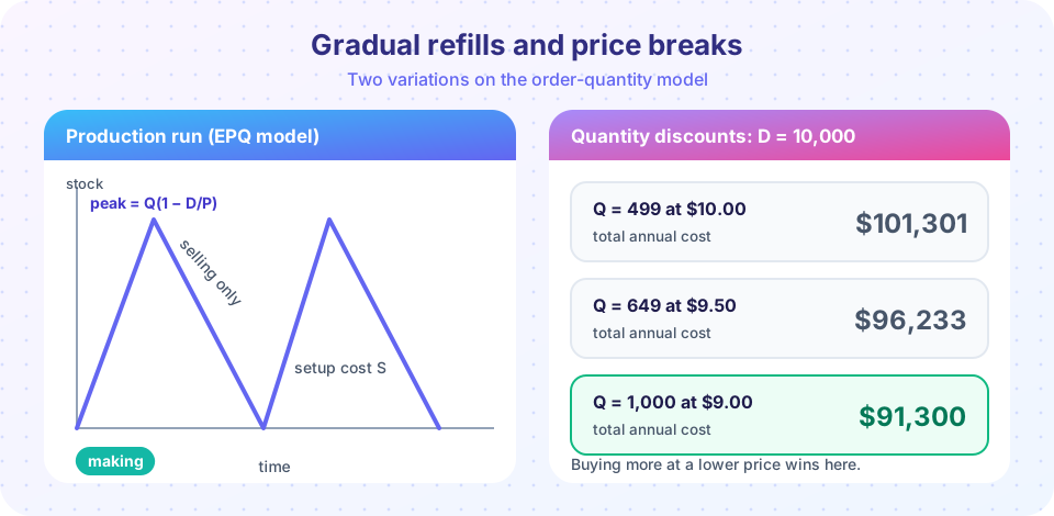
Replace the sudden delivery by a machine that makes P units per year. While it runs, stock grows at a net rate of P − D (it produces P and customers take D). When the run ends, stock falls at rate D until it is time for the next run. The picture is a sawtooth with a gentle upward slope.
For a run of Q units:
- Making
Qunits takesQ / Pyears. In that time stock rises by(P − D) × Q / P = Q(1 − D/P). That is the maximum stock. - Because stock rises and falls in straight lines, the average stock is half of the maximum:
Q(1 − D/P) / 2.
So the total yearly cost is
TC(Q) = D·S / Q + H·Q(1 − D/P) / 2
The structure is identical to EOQ with one change: the holding cost is multiplied by (1 − D/P). The same balancing argument gives
Q* = √(2DS / (H(1 − D/P))) and TC* = √(2DSH(1 − D/P))
When P is huge compared with D, the factor (1 − D/P) approaches 1 and EPQ becomes EOQ. When P only just exceeds D, the factor approaches 0 and runs become very long: it is almost better to produce continuously.
A worked example
A plant fills a warehouse with a polish, selling 12,000 cases a year. The line can make 48,000 cases a year. Each setup costs $200, and holding costs $2 per case per year.
D/P = 12,000 / 48,000 = 0.25, so1 − D/P = 0.75.Q* = √(2 × 12,000 × 200 / (2 × 0.75)) = √3,200,000 ≈ 1,789cases.- Maximum stock:
1,789 × 0.75 ≈ 1,342cases. The warehouse never needs room for the full batch. - Run length:
1,789 / 48,000 ≈ 0.037years, about 13.6 days of production. - Runs per year:
12,000 / 1,789 ≈ 6.7. - Minimum yearly cost:
√(2 × 12,000 × 200 × 2 × 0.75) ≈ $2,683.
Press Run (or Ctrl + Enter) to see the result here.
Program input · what you'd type while the program runs
Type the answers before you press Run, one per line. Each time the program reads a line (with input()), it gets the next line from this box.
The last loop shows the limit: as P grows, Q* approaches the EOQ value of √(2DS/H) ≈ 1,549.
Quantity discounts
Now return to purchasing. A supplier offers, for a product you use 10,000 times a year:
| Order size | Unit price |
|---|---|
| 1 to 499 | $10.00 |
| 500 to 999 | $9.50 |
| 1,000 or more | $9.00 |
Each order costs S = $40, and holding costs 20 percent of the unit price per year (H = 0.2 × price). Now the purchase cost D × price does depend on the decision, so we must include it:
TC(Q) = D × price + D·S / Q + H·Q / 2, with H = 0.2 × price.
The all-units discount procedure
- For every price level, compute its own EOQ using that level's holding cost.
- If that EOQ lies inside the level's allowed range, it is a candidate. If it is too small, move up to the lowest quantity of the range. If it is too large, the level cannot be used.
- Compute the total cost of every candidate (including the purchase cost) and choose the smallest.
For our numbers: at $10, the EOQ is √(2 × 10,000 × 40 / 2) ≈ 632, which is above the allowed maximum of 499, so we use Q = 499. At $9.50 the EOQ is √(2 × 10,000 × 40 / 1.9) ≈ 649, inside the range 500 to 999. At $9.00 the EOQ is about 667, below the minimum 1,000, so we use Q = 1,000.
The totals are roughly $101,301, $96,233 and $91,300. The biggest order wins by a wide margin because the purchase bill is by far the largest part: saving 50 cents on 10,000 units is worth $5,000 a year, far more than the extra holding cost.
Press Run (or Ctrl + Enter) to see the result here.
Program input · what you'd type while the program runs
Type the answers before you press Run, one per line. Each time the program reads a line (with input()), it gets the next line from this box.
Incremental discounts
A different scheme gives the lower price only for the extra units above the threshold. The cost function is then a piecewise-linear curve and the same step-by-step method works, but each price level needs its own fixed purchase-cost adjustment. The idea is the same: compute each piece, clamp into range and compare.
A visual check
The plot compares the yearly cost curves of the three price levels. Only the solid part of each curve is allowed.
Press Run (or Ctrl + Enter) to see the result here.
Program input · what you'd type while the program runs
Type the answers before you press Run, one per line. Each time the program reads a line (with input()), it gets the next line from this box.
Choosing between the models
How do you know which model fits? Check the assumptions about the arrival of stock. If a supplier delivers a whole truckload on one day, EOQ applies. If your own line fills the warehouse while you sell from it, EPQ applies. The difference can be large: for the same data (D = 12,000, S = $200, H = $2) the EOQ is about 1,549 units, while the EPQ with a production rate of 48,000 is about 1,789 units. The EPQ run is bigger because the stock never reaches the full batch size, so large runs are cheaper to hold. It also costs less per year, about $2,683 against $3,098 for the EOQ. Using the wrong model would give the wrong batch and the wrong cost forecast, though in practice the penalty is small because the cost curves are flat.
A last practical point: price breaks and setup costs often work against each other. A large order earns a low price but ties up cash, so many firms add a cost of capital to the holding rate. In the discount example the holding rate of 20 percent of the price includes that cost. Raising the rate to 30 percent would move the best choice toward smaller orders, and it is a useful what-if to try in the solver above.
Common misconceptions
"The discounted EOQ is the answer." An EOQ computed at a lower price may fall below the quantity needed to earn that price. You must check that it is feasible, or move to the break quantity.
"Bulk buying is always cheaper." It is cheaper only when the savings on the purchase bill exceed the extra holding (and risk of spoilage or obsolescence). With a large holding rate or a perishable product the small order can win.
"EPQ needs a separate theory." It is EOQ with the holding cost scaled by 1 − D/P.
Check your understanding
Quick check · 5 questions
of 5 answered You scored / 5 · perfect!
-
1. In the EPQ model, what is the maximum stock for a run of Q units?
Stock rises by Q(1 − D/P) during the run because customers keep buying while the machine produces. -
2. When the production rate P becomes very large, the EPQ approaches what?
The factor 1 − D/P tends to 1, so the formula becomes the EOQ formula. -
3. D = 6,000, P = 24,000, S = $100, H = $3. What is the EPQ?
Q* = √(2 × 6,000 × 100 / (3 × 0.75)) = √(1,200,000 / 2.25) = √533,333 ≈ 730. -
4. Under all-units discounts, what must you do with a level whose EOQ is below its price break?
If the level EOQ is too small, the lowest feasible quantity at that price is the break itself, and its total cost is compared with the other candidates. -
5. Why do purchase costs matter in the discount model but not in basic EOQ?
When unit price depends on order size, D × price changes between options and must be included.
Summary
- EPQ is EOQ for stock that fills gradually: holding cost is scaled by
1 − D/P, andQ* = √(2DS / (H(1 − D/P))). - Peak stock is
Q(1 − D/P), so a factory needs less space than the batch size suggests. - For all-units discounts, find each level's EOQ, clamp it into the allowed range, add the purchase cost and compare totals.
- The purchase bill is often the biggest term, so bulk prices frequently win.
Track your progress
Create a free account to tick off lessons and pick up where you left off on any device.
of Operations Research lessons completed