


















Lesson 37 of 46 · Model Validation and Communication
Fitting models by least squares
Fit lines and nonlinear curves to data with least squares, read residual plots and R-squared, estimate parameter uncertainty and avoid overfitting with held-out data.
You have a model with unknown constants, such as the cooling constant k of a cup of coffee, and some measurements. Which values of the constants make the model agree best with the data? Choosing them is called fitting or calibration, and the standard tool, going back to Legendre (1805) and Gauss, is least squares: choose the constants that make the sum of the squared errors as small as possible. In this lesson you will fit a line by hand, fit a nonlinear model with SciPy, look at what the leftover errors reveal, and see how an over-flexible model can fool you.
What you will learn
- What a residual is and why we square it.
- The closed-form least-squares line and the meaning of R².
- How to fit a nonlinear model and get uncertainty for its parameters.
- How training and test errors reveal overfitting.
Key terms
Residual: observed value minus model value, eᵢ = yᵢ − ŷᵢ.
Sum of squared errors (SSE): Σ eᵢ², the quantity least squares minimizes.
R² (coefficient of determination): the fraction of the variation in y explained by the model, 1 − SSE/SST.
Test set: data kept aside and not used for fitting, used to judge predictions.
Least squares for a straight line
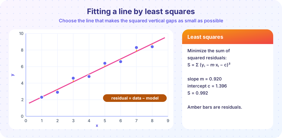
Given points (xᵢ, yᵢ) and the model ŷ = m·x + c, the residuals are eᵢ = yᵢ − m·xᵢ − c. We minimize S = Σ eᵢ². Squaring makes all errors positive, punishes big misses more than small ones, and gives a smooth function whose minimum we can find with calculus. Setting ∂S/∂m = 0 and ∂S/∂c = 0 gives
m = Σ (xᵢ − x̄)(yᵢ − ȳ) / Σ (xᵢ − x̄)² and c = ȳ − m·x̄.
For the eight points in the picture (x = 1, …, 8, y = 2.3, 2.9, 4.6, 4.8, 6.4, 6.6, 8.3, 8.4) this gives m ≈ 0.920 and c ≈ 1.396, with S ≈ 0.99. The line always passes through the centre point (x̄, ȳ), and the residuals always sum to zero.
To judge how good the fit is, compare SSE with the total variation SST = Σ (yᵢ − ȳ)²: R² = 1 − SSE/SST. An R² of 0.99 means the line explains 99 percent of the variation. But R² alone does not prove the model is right: a curved relationship can still give a high R² with a straight line. Always look at the residuals themselves.
Residual plots
If the model is adequate, residuals should look like random scatter around zero with no pattern. A curve in the residuals means the model has the wrong shape. A fan shape (spread growing with x) means the noise is not constant. A few huge residuals mean outliers that deserve investigation, not automatic deletion.
Press Run (or Ctrl + Enter) to see the result here.
Program input · what you'd type while the program runs
Type the answers before you press Run, one per line. Each time the program reads a line (with input()), it gets the next line from this box.
Fitting a nonlinear model
Most models in this course are not straight lines. Take Newton's cooling law from Chapter 5, T(t) = T_room + ΔT·e^(−k·t). It is nonlinear in k, so there is no formula; we minimize SSE numerically. SciPy's curve_fit does this and also returns a covariance matrix whose diagonal gives the variance of each parameter estimate. The square roots are the standard errors, a measure of how well the data pin down each parameter.
Here we invent data from known values (T_room = 20, ΔT = 70, k = 0.05) plus noise, so we can see whether the fit recovers the truth. In real life you would not know the truth, which is why the standard errors matter.
Press Run (or Ctrl + Enter) to see the result here.
Program input · what you'd type while the program runs
Type the answers before you press Run, one per line. Each time the program reads a line (with input()), it gets the next line from this box.
Common misconceptions
"A high R² means the model is correct." It only says the fitted curve is close to the data. A wrong-shaped model can have a high R² over a limited range and fail outside it.
"Delete the points that don't fit." Outliers can be errors, but they can also be the most interesting facts. Investigate before deleting, and say what you removed.
"Correlation proves the model's cause." Least squares finds the best curve of the chosen shape. It does not know whether the relationship is causal.
Overfitting and the test set
If you let a model have as many adjustable constants as data points, it can pass through every point exactly and have SSE = 0. A polynomial of degree 9 can do that with ten points. But it is fitting the noise, so its wiggles between the points are inventions. The cure is to hold out data: fit on a training set, then measure the error on a separate test set. The training error always falls as the model gets more flexible, while the test error typically falls and then rises again. The best model is near the minimum of the test error.
Press Run (or Ctrl + Enter) to see the result here.
Program input · what you'd type while the program runs
Type the answers before you press Run, one per line. Each time the program reads a line (with input()), it gets the next line from this box.
Check your understanding
Quick check · 5 questions
of 5 answered You scored / 5 · perfect!
-
1. What is a residual?
Residual = data - model. -
2. Why does least squares square the errors?
Squares avoid cancellation of positive and negative errors and give calculus-friendly minimization. -
3. A least-squares line fits data with R-squared = 0.97. What can you conclude?
R-squared measures closeness, not correctness of the model's shape. -
4. As model flexibility increases, the training error:
A more flexible model can always follow the training data more closely. -
5. Why use a test set?
Test error exposes overfitting that training error hides.
Summary
- Least squares minimizes
Σ residual²; for a line,m = Sxy/Sxxandc = ȳ − m·x̄. R² = 1 − SSE/SSTmeasures closeness; residual plots test the shape.curve_fitfits nonlinear models and gives standard errors for the parameters.- Hold out test data to detect overfitting.
Track your progress
Create a free account to tick off lessons and pick up where you left off on any device.
of Mathematical Modelling lessons completed