


















Lesson 16 of 46 · Discrete Dynamical Models
Discrete Models: Overview
Chapter 4 overview: models that change in steps, written as rules x(n+1) = f(x(n)). Meet savings, loans, populations and Fibonacci, with runnable examples.
Many things in life happen in steps. Interest is added once a month. Insects have one generation per summer. A game updates its world 60 times a second. A loan is paid down by instalments. For these situations the cleanest model is not a curve in continuous time but a rule that turns today's state into tomorrow's.
This chapter develops that idea: the rule, the sequence it creates, the special states where nothing changes, and the surprising behavior (including chaos) that even simple rules can produce.
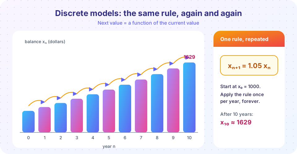
The big picture
A discrete dynamical model has three ingredients:
- a state
xₙ(a number, or a list of numbers) at stepn = 0, 1, 2, ... - an update rule
xₙ₊₁ = f(xₙ)that gives the next state from the current one - an initial condition
x₀
Together they generate the whole future: x₀, x₁ = f(x₀), x₂ = f(x₁), .... Such a rule is called a difference equation or recurrence relation. If f is simple, you can often find a formula for xₙ; if not, you can always run it on a computer.
Three questions run through the chapter:
- What happens in the long run? Growth, decay, settling to a steady state, cycling, or chaos?
- Where are the equilibria (fixed points), states with
f(x*) = x*? - Are those equilibria stable: if you nudge the system, does it return?
Some real examples with their rules:
| Situation | Rule | Notes |
|---|---|---|
| Savings at 5% a year | xₙ₊₁ = 1.05 xₙ |
Pure growth |
Loan with monthly payment P and monthly rate i |
xₙ₊₁ = (1 + i) xₙ − P |
Balance shrinks if P is large enough |
| Rabbit pairs (Leonardo of Pisa, 1202) | Fₙ₊₁ = Fₙ + Fₙ₋₁ |
Depends on two past values: second order |
| Insect generations | xₙ₊₁ = r xₙ (1 − xₙ) |
The logistic map: crowded populations |
Step by step
Long-run questions
Tools ahead
What this chapter covers
| Lesson | You will learn |
|---|---|
| Difference Equations and Their Solutions | Linear rules, closed forms, equilibria, loans and mortgages |
| The Logistic Map and Chaos | Crowded populations, cobweb diagrams, stability, period doubling |
| Matrix Models: Leslie and Markov | Age-structured populations and long-run growth rates |
| Chapter 4 Review | A cobweb cheat sheet and a longer quiz |
Try it
Write the rule as code. One function holds the update rule; a loop applies it. This pattern, state in, next state out, is how nearly every discrete model is simulated.
Press Run (or Ctrl + Enter) to see the result here.
Program input · what you'd type while the program runs
Type the answers before you press Run, one per line. Each time the program reads a line (with input()), it gets the next line from this box.
The next demo lets you change the growth factor r in x(n+1) = r · x(n) and watch ten steps. Try values just below, at and just above 1.
Check your understanding
Quick check · 4 questions
of 4 answered You scored / 4 · perfect!
-
1. In a discrete dynamical model, the update rule gives:
x(n+1) = f(x(n)) turns today's state into tomorrow's. -
2. What is a fixed point of the rule f?
If the state is x* and f(x*) = x*, the next state equals the current one forever. -
3. The Fibonacci rule F(n+1) = F(n) + F(n-1) depends on how many past values?
It uses the last two terms, so it is a second-order recurrence. -
4. A savings account follows x(n+1) = 1.05 x(n). Which long-run behavior do you expect?
Multiplying by a factor above 1 each step makes the balance grow without bound.
Summary
- A discrete model is a state, an update rule
xₙ₊₁ = f(xₙ)and an initial condition. - Key questions: long-run behavior, equilibria
f(x*) = x*and their stability. - Examples: savings, loans, Fibonacci rabbits, crowded populations.
- Code pattern: one function for the rule, one loop that applies it.
Track your progress
Create a free account to tick off lessons and pick up where you left off on any device.
of Mathematical Modelling lessons completed