


















Lesson 26 of 46 · Optimization Models
Chapter 6 overview: optimization models
See how optimization models work: choose decisions, respect constraints and aim at an objective, with a preview of calculus, linear programming and gradient descent.
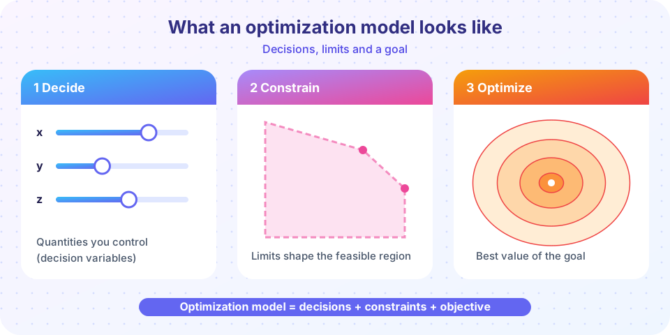
Many real questions are not "what will happen?" but "what should we do?". How many seats should a bus have? What shape of can uses the least metal? How many tables and chairs should a workshop build today? These are optimization problems: out of all the choices that are allowed, find the best one. In this chapter you will learn to write such questions as models and solve them with calculus, linear programming and gradient descent.
What you will learn
- The three ingredients of every optimization model: decision variables, constraints and an objective.
- How to tell a good formulation from a bad one before touching any numbers.
- When to use calculus, when to use linear programming and when to use an iterative search.
- Why a mathematical optimum is the start of a conversation, not the end.
Key terms
Decision variables: the quantities you are free to choose.
Objective function: the single number you want to make as large (profit) or as small (cost) as possible.
Constraints: equations or inequalities that the choices must satisfy.
Feasible region: the set of all choices that satisfy every constraint.
Three ingredients
Suppose you are designing a fence for a rectangular vegetable bed with 40 m of fencing. The decision variables are the width x and the length y. The constraint is that the fence is 40 m long: 2x + 2y = 40. The objective is the area A = x·y, which you want to maximize. Substituting y = 20 − x gives A = x(20 − x), a parabola with its peak at x = 10: a 10 m by 10 m square, area 100 m².
Notice how little arithmetic that took, and how much of the work was formulating the problem. The first lesson of this chapter, after this overview, is about exactly that.
Decide
Constrain
Optimize
Check
What each lesson covers
- Calculus and design: set the derivative to zero for fences, cans and prices.
- Linear programming models: many linear constraints, corner points and shadow prices.
- Gradient descent and fitting: searching downhill when there is no formula, and why learning rates matter.
- Chapter review: a poster, a recap table and ten questions.
Try it
A computer can always try many values. This demo finds the best fence by a brute-force search and compares it with the calculus answer.
Press Run (or Ctrl + Enter) to see the result here.
Program input · what you'd type while the program runs
Type the answers before you press Run, one per line. Each time the program reads a line (with input()), it gets the next line from this box.
Check your understanding
Quick check · 4 questions
of 4 answered You scored / 4 · perfect!
-
1. Which of these is a decision variable in a fence-design problem?
Decision variables are the things you can choose, such as the width and length. -
2. What is the feasible region?
A choice is feasible if it obeys all the constraints; the feasible region is the set of such choices. -
3. With 40 m of fence and a rectangular bed, which dimensions give the largest area?
A = x(20 - x) is largest at x = 10, giving 100 square metres. -
4. Why should you test an optimum against the real situation?
An optimum is only optimal for the model you wrote; missing constraints or goals can make it useless in practice.
Summary
- An optimization model has decision variables, constraints and an objective.
- The hard part is formulation: choosing variables, writing limits and stating one goal.
- Calculus, linear programming and gradient descent fit different problem shapes.
- Check the answer against the real world and ask "what if a number changes?".
Next: Calculus and design
Track your progress
Create a free account to tick off lessons and pick up where you left off on any device.
of Mathematical Modelling lessons completed